This is Part 2 of a 3-part series to The Complete Guide To Sentiment Analysis with Ludwig. Part 1 shows how to load the dataset and how to obtain baseline Ludwig models. This part will show how to work with Transformer encoders like BERT and how to compare all the models using Ludwig.

You can follow along with the code through the Colab notebook.

Authors: Kanishk Kalra, Michael Zhu, Elias Castro Hernandez, and Piero Molino

Thanks to Debbie Yuen for the Images

III. BERT

BERT is a state-of-the-art model introduced in BERT: Pre-training of Deep Bidirectional Transformers for Language Understanding by Devlin et al. (2019), that uses the Transformer architecture Attention is all you need by Vaswani et al. BERT is a family of models made of a deep stack of self-attention-based transformer layers pre-trained using a Masked Language Model objective over a large corpus, which consists in reading a sentence from the corpus, masking-out some words from it and teaching the model to predict the masked words back. Fine-tuning the pre-trained BERT representations on specific datasets allows us to achieve close to state-of-the-art performance in several sentence-level and token-level tasks.

Building BERT Using Ludwig

There’s no major difference between Ludwig configuration for BERT and the ones we defined in Part 1 for the Parallel CNN and bi-LSTM. The only minor changes are in the input_featuresand the training parameters.

In the input_features, we change the encoder to BERT ('encoder': 'bert') and remove all the embedding related parameters, not needed for this type of architecture. All the other parameters are kept the same for this section. While fine-tuning a BERT encoder, we suggest using a smaller learning rate ('learning_rate': 0.00002) and smaller batch size('batch_size': 16) to avoid out-of-memory issues because of the high memory consumption of BERT. Since BERT is larger than the previous models we trained and takes a lot of time per epoch (~1.25 hrs/epoch), we recommend setting the number of epochs to 2 ('epochs': 2) when working on Colab as it is sufficient to achieve good results on SST and avoids loss of metadata in case Colab gets disconnected.

config = {
    'input_features': [{
        'name': 'text', 
        'type': 'text',  
        'encoder': 'bert'
    }],  
    'output_features': [{'name': 'label', 'type': 'category'}],    
    'training': {
        'batch_size': 16,
        'decay': True,
        'trainable': True,
        'learning_rate': 0.00002,
        'epochs': 2
    }
}
 
print("Instantiating LudwigModel...")
bert = LudwigModel(config, logging_level=logging.DEBUG)
 
print("Training Model...")
train_stats_bert, _, _ = bert.train(
    training_set=train_data, 
    validation_set=validation_data, 
    test_set=test_data,    
    model_name='bert',
    skip_save_processed_input=True
    )

Visualizing and Interpreting BERT’s Results

Now that we’ve fine-tuned BERT for SST-5, let’s visualize the learning curves with the help of the training statistics returned intrain_stats_bert.

learning_curves(train_stats_bert, output_feature_name='label', model_names='bert')

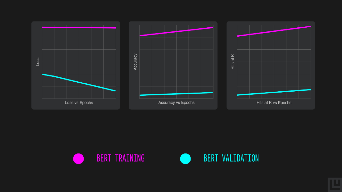
Just a glimpse of the learning curves suggests that BERT requires little to no fine-tuning to perform at par or even better in comparison to the other two models (Parallel CNN, Bi-LSTM) we trained previously, as illustrated in the epochs vs accuracy graph where already at the end of the first epoch the validation accuracy is above 0.5.

We observe that the model achieved a maximum validation accuracy of 53.8% at epoch 2, higher than both the earlier models. To confirm the good results obtained on the validation set, let’s use some tools built into Ludwig to evaluate and compare BERT with the previous models using the held-out test set.

Model Evaluation and Comparisons

So far we have seen how different models perform on the training and validation set of SST-5 dataset, but what we really care about is how well do they generalize on the test set. Ludwig provides a very intuitive way for evaluating the models on the test data using the evaluate method. The method returns test statistics, predictions for the model evaluated and the output directory where the results get stored. The performance of the models can be compared head to head using the compare_performance visualization method that plots the performance of each of the models in the form of bar charts and the predictions can be compared in the form of donut plots using the compare_classifiers_predictions visualization method.

Let’s first evaluate the models on the test set. It’s noteworthy to mention that Colab might remove the models from the memory to free up space, but we can seamlessly load the trained models back from their respective directories with the load method that Ludwig provides.

parallel_cnn = LudwigModel.load('/content/results/api_experiment_parallel_cnn/model')
test_stats_parallel_cnn, predictions_parallel_cnn, _ = parallel_cnn.evaluate(
  dataset=test_data,
  skip_save_predictions=False,
  collect_predictions=True,
  output_directory='test_results/parallel_cnn'
  )

bi_lstm = LudwigModel.load('/content/results/api_experiment_bi_lstm/model')
test_stats_bi_lstm, predictions_bi_lstm, _ = bi_lstm.evaluate(
    dataset=test_data,
    skip_save_predictions=False,
    collect_predictions=True,
    output_directory='test_results/bi_lstm'
    )

bert = LudwigModel.load('/content/results/api_experiment_bert/model')
test_stats_bert, predictions_bert, _ = bert.evaluate(
    dataset=test_data,
    skip_save_predictions=False,
    collect_predictions=True,
    output_directory='test_results/bert'
    )

Head to Head Performance Comparison on Test Set

Let’s now compare the performance of the models on the test set across accuracy and Hits@3 metric in the form of horizontal bar-charts obtained with the compare_performance function.

compare_performance([test_stats_parallel_cnn, test_stats_bi_lstm, test_stats_bert],
                    output_feature_name='label', model_names=['Parallel CNN', 'Bi-LSTM', 'BERT'])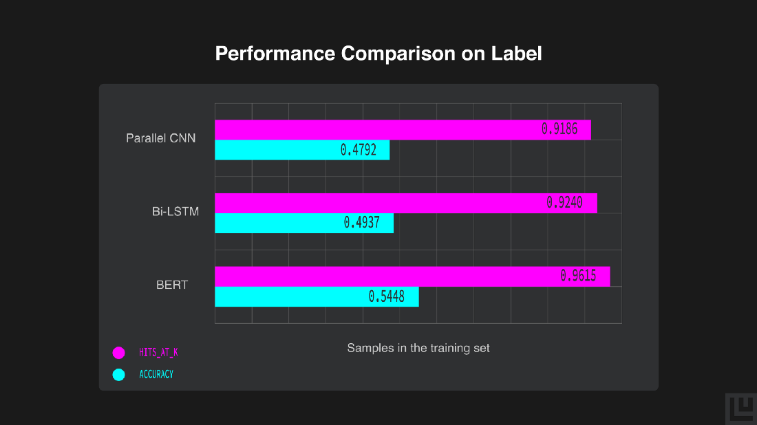

We can see how BERT performs better on the sentiment analysis task as compared to the other two models, with an accuracy of 54.48 %.

Even though BERT performs better, there’s a trade-off between the accuracy of the predictions and the time required to calculate them. We created a function to obtain 5 shuffled test sets in order to average the elapsed prediction time.

import time

def shuffled_dataset(test_data, num_shuffles=5):
  test_set = []
  for i in range(num_shuffles):
    test_set.append(test_data.sample(frac=1).reset_index(drop=True))
  return test_set

shuffled_testset = shuffled_dataset(test_data)

elapsed_time = []
for i in shuffled_testset:
  start = time.time()
  prediction_parallel_cnn, _ = parallel_cnn.predict(dataset=i, batch_size=1)       
  end = time.time()
  elapsed_time.append((end-start)/len(i))

prediction_time_parallel_cnn = sum(elapsed_time)*1000/len(elapsed_time)
print(f'Avg Time Elapsed: {prediction_time_parallel_cnn} ms')

We see that Parallel CNN takes 1.25ms on an average per prediction.

elapsed_time = []
for i in shuffled_testset:
  start = time.time()
  prediction_bi_lstm, _ = bi_lstm.predict(dataset=i, batch_size=1)       
  end = time.time()
  elapsed_time.append((end-start)/len(i))

prediction_time_bi_lstm = sum(elapsed_time)*1000/len(elapsed_time)
print(f'Avg Time Elapsed: {prediction_time_bi_lstm} ms')

The Bi-LSTM takes 3.69ms on an average per prediction.

elapsed_time = []
for i in shuffled_testset:
  start = time.time()
  prediction_bert, _ = bert.predict(dataset=i, batch_size=1)       
  end = time.time()
  elapsed_time.append((end-start)/len(i))

prediction_time_bert = sum(elapsed_time)*1000/len(elapsed_time)
print(f'Avg Time Elapsed: {prediction_time_bert} ms')

Finally, BERT takes 8.62ms on an average per prediction.

from tabulate import tabulate

model_names = ['Parallel CNN', 'Bi-LSTM', 'BERT']
test_accuracy = [ 0.4792, 0.4937, 0.5448]
prediction_latency = [prediction_time_parallel_cnn, prediction_time_bi_lstm, prediction_time_bert]

header = ['Model Name', 'Test Accuracy', 'Prediction Latency (ms)']
print(tabulate([*zip(model_names, test_accuracy, prediction_latency)], headers=header, tablefmt='grid'))

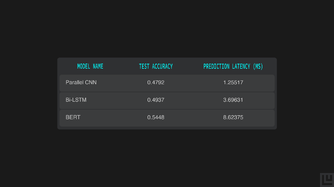
We can distinctly see the difference in how BERT performs better on the sentiment analysis task with an accuracy of 54.48%, although predicting using it takes 8.62ms while predicting using the Bi-LSTM take 3.69ms. Depending on deployment constraints you can choose to run a faster, but less accurate model or a slower but more accurate one.

Comparing Test Set Predictions

Now, let’s visualize the test predictions for each of the models.

After comparing the performance of the models, let’s use Ludwig’s visualization module to get detailed insights into predictions by comparing them pairwise to understand how much they align or differ using the donut plot generated by the compare_classifiers_predictions visualization function.

metadata_parallel_cnn = load_json('/content/results/api_experiment_parallel_cnn/model/training_set_metadata.json')

compare_classifiers_predictions([np.array(predictions_parallel_cnn['label_predictions'], dtype=int),
                                np.array(predictions_bi_lstm['label_predictions'], dtype=int)],
                                ground_truth=np.array(test_data['label']), labels_limit=5,
                                output_feature_name='label', metadata=metadata_parallel_cnn,
                                model_names=['Parallel CNN', 'Bi-LSTM'])

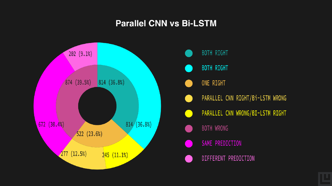
The inner donut illustrates a generic estimate of the models’ predictions — both correct (36.8%), both incorrect (39.5%), either of them correct (23.6%). The outer donut represents a detailed outline of the inner estimates — both correct (36.8%), both incorrect yet same (30.4%) or different (9.1%), Parallel CNN being correct and Bi-LSTM being incorrect (11.1%) and vice-versa (12.5%).

The plot shows that the model behaves similarly because of the big green and red areas, and that the bi-LSTM outperforms the Parallel CNN, although there’s still an 11% of data points where the Parallel CNN are correct and the bi-LSTM ones are wrong.

metadata_bert = load_json('/content/results/api_experiment_bert/model/training_set_metadata.json')

compare_classifiers_predictions([np.array(predictions_bi_lstm['label_predictions'], dtype=int),
                                np.array(predictions_bert['label_predictions'], dtype=int)],
                                ground_truth=np.array(test_data['label']), labels_limit=5,
                                output_feature_name='label', metadata=metadata_bert,
                                model_names=['Bi-LSTM', 'BERT'])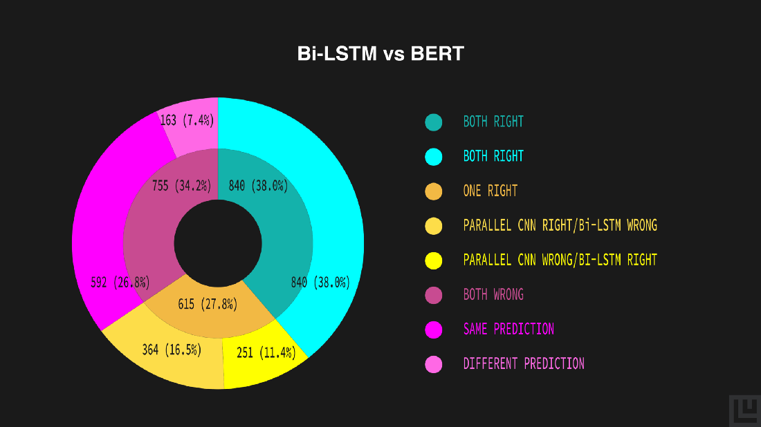

Similarly, from the above donut plot, we can compare Bi-LSTM’s and BERT’s predictions. According to the plot, a generic estimate of the models’ predictions — both correct (38.0%), both incorrect (34.2%), either of them correct (27.8%) and a detailed outline of the generic estimates — both correct (38.0%), both incorrect yet same (26.8%) or different (7.4%), Bi-LSTM being correct and BERT being incorrect (11.4%) and vice-versa (16.5%).

In this case, the predictions of the models are more diverse with a larger yellow area, but also in this case, despite BERT being more accurate, there’s still an 11% of data points that the bi-LSTM predicts correctly and BERT does not.

Testing model’s predictions on Unseen data

Let’s use the model we evaluated as most accurate and most generalizable to predict the sentiment of a movie review we made-up.

# text for predicting
texts = ["This movie is amazing!", 
         "I hated the movie so much.", 
         "The special effects were ok, but the story was nothing special."]

# converting the text into dataframes
texts_df = pd.DataFrame({'text': texts})

# predicting using our best model
predictions, _ = bert.predict(dataset=texts_df)

# ids to labels
labels = []
for prediction in predictions['label_predictions']:
  labels.append(idx2class[int(prediction)])

# processing the ids, labels and text into a single dataframe
predictions_df = texts_df.assign(class_id=predictions['label_predictions'], class_label=labels)

pd.set_option('display.max_colwidth', None)  
predictions_df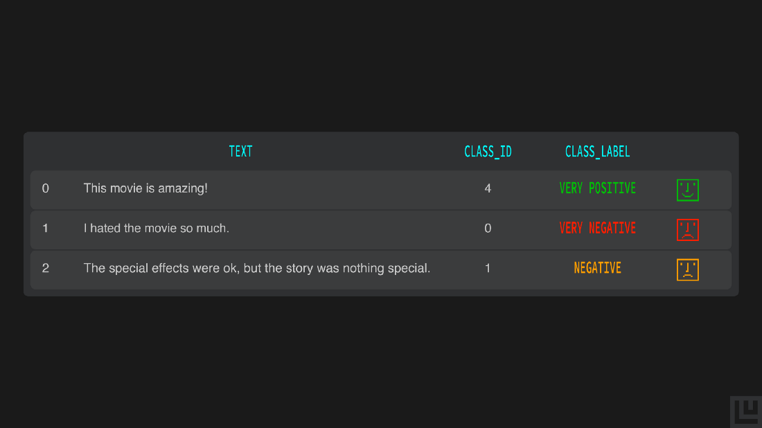

Our BERT Ludwig model predicts the correct sentiment of those made-up reviews.Want to know how you can easily optimize the hyperparameters of your Ludwig models? Check out Part 3 of the series, where we discuss hyperparameter optimization. Missed out the Part 1, find it here.

We encourage you to check out the documentation to learn more and to become engaged with the Ludwig open source community. We aim to make deep learning free and accessible to all. Also, follow Ludwig on Twitter to stay afloat with all news and developments. We hope you’ll join us.