This is the third article of a 3-part series about using Ludwig to perform Sentiment Analysis on the Stanford Sentiment Treebank dataset. Part 1 provides an introduction to the dataset and shows how to train two types of models (Bi-LSTM and parallel-CNN). Part 2 describes the BERT model and how to use it in Ludwig. You can follow along with the code through our Colab notebook.

Authors: Michael Zhu, Kanishk Kalra, Elias Castro Hernandez, and Piero Molino

Images thanks to Debbie Yuen

Introduction

In this article, we will be using Ludwig — a deep learning toolkit based on Tensorflow — to perform hyperparameter optimization on a Recurrent Neural Network used for Sentiment Analysis.

What are hyperparameters and what is hyperparameter optimization?

In deep learning, the parameters are the weights learned during the model training process. If we imagine a model to be a matrix that transforms an input vector (i.e. flattened image vector) into an output vector (i.e. vector of categories) so that output = matrix ⋅ input, then the parameters would be the values of the matrix that are updated throughout the training process (i.e. by some form of stochastic gradient descent). In reality, a deep learning model is made of several tensors of different shapes, and the parameters are the values of all those tensors.

Hyperparameters are values that define either the architecture of the model (like the size of some layers or the type of activation) or control the data processing and the training process (like the learning rate or the batch size). They are usually set by the user before training. We will go over some examples of hyperparameters that are commonly used below.

Hyperparameter optimization is the process of picking the best possible hyperparameters so that the training process achieves optimal performance. In its simplest form — grid search — this consists of training a model multiple times with different hyperparameter values obtained by exhaustively enumerating all combinations and picking the best performing set of hyperparameters. Another option is to use random search, which consists of sampling hyperparameters at random from specified ranges. There are, although, many more interesting ways to sample hyperparameters, like Bayesian optimization and evolutionary strategies. In this article we will use random search for simplicity, but Ludwig also supports grid search and Bayesian optimization samplers.

What hyperparameters can we optimize and what do they do?

Our goal is to find the best hyperparameters for the Recurrent Neural Network we trained in Part 1, so we selected a mix of training and architecture hyperparameters:

Learning rate: tells the optimizer how much to update the weights at each step (0.0≤𝜅≤1.0).

• If learning rate is too large, 𝜅→1.0, then gradient descent may never converge to a minimum.
• If learning rate is too small, 𝜅→0.0, then the model may take too long to train and may end up stuck in local minima.

State size: the size of the hidden state of the RNN.

• Larger state size will allow each RNN cell to pass along more information at each step and will increase the model capacity, but will also increase computation time and potentially make the model more prone to overfitting.

Number of encoder layers: more layers may result in higher accuracy because of increased model capacity, but will also be more computationally expensive and may lead to overfitting.

RNN cell type:

• Vanilla RNN: processes input and hidden state with a single weight matrix. The vanilla RNN cell has issues with exploding and vanishing gradients. For more details on RNNs refer to this paper by Paul Rodriguez, Janet Wiles & Jeffrey L. Elman.
• Gated Recurrent Units (GRU): GRU cells include a forget gate that updates the hidden state by removing unnecessary information. For more details on GRU’s refer to this paper by Kyunghyun Cho et al.
• Long Short Term Memory (LSTM): LSTM cells use an additional cell state that is passed between cells along with the hidden state. LSTMs have 3 gates: input gate, forget gate, and output gate which are used to update the cell state and calculate new hidden states. For more details on LSTM’s refer to this paper by Hochreiter and Schmidhuber.

Bidirectionality:

• One directional sequence models generally process the input in first to last order.
• Bidirectional sequence models act like a one directional sequence model, with the addition of a second hidden layer that processes the input in the order of last to first.

Ludwig Hyperopt Module

Ludwig implements hyperparameter optimization through its hyperopt module. Hyperopt consists of three main phases: sampling, training, and evaluation. It first samples a set of hyperparameters using a user-defined sampling strategy (i.e. random sampling), and then performs training with those hyperparameters. Hyperopt uses the validation and test data to evaluate the performance of the hyperparameters, and then repeats this cycle by sampling a new set of hyperparameters. Users can also define different executors to run the process in parallel and on a remote Kubernetes cluster, but for simplicity we will use the simple serial executor

Let’s install Ludwig along with a few more dependencies that we will need in order to use the hyperopt module.

$ pip install ludwig[hyperopt]

Configuration

In order to use the hyperopt functionality we need to write a configuration which includes an hyperopt section in which we declare to Ludwig the specification of the hyperparameter optimization we want to run. In the configuration below we are trying to optimize for 4 hyperparameters: learning rate, state size, RNN cell type, and the number of encoder layers. The configuration is the same as the previous parts from this series with the addition of the hyperopt section.

config = {
    'input_features': [{
        'name': 'text',
        'type': 'text',
        'level': 'word',
        'encoder': 'rnn',
        'cell_type': 'lstm',
        'bidirectional': True,
        'pretrained_embeddings': '/content/glove/glove.6B.300d.txt',
        'embedding_size': 300,
        'preprocessing': {
            'word_vocab_file': '/content/glove/glove.6B.300d.txt'
        }
    }],
    'output_features': [
        {'name': 'label', 'type': 'category'}
    ],
    'training': {
        'decay': True,
        'learning_rate': 0.001,
        'validation_field': 'label',
        'validation_metric': 'accuracy'
    },
    'hyperopt': {
        'goal':'maximize',
        'output_feature': 'label',
        'metric': 'accuracy',
        'split': 'validation',
        'parameters': {
            'training.learning_rate': {
                'type': 'float',  
                'low': 0.000005,
                'high': 0.001,
                'steps': 4,
                'scale': 'log'
            },
            'utterance.state_size':{
                'type': 'int',
                'low': 300,
                'high': 900,    
                'steps': 3
            },
            'utterance.cell_type': {
                 'type': 'category',
                 'values': ['rnn', 'gru', 'lstm']
             },
            'utterance.num_layers': {
                 'type': 'int',
                 'low': 1,
                 'high': 5
            },
        },
        'sampler': {
            'type': 'random',
            'num_samples': 80
        },
        'executor': {
            'type': 'serial'
        }
    }
}

The above config tells Ludwig to run 80 random samples with the goal of maximizing the validation accuracy of the output feature called label.

To learn more about the hyperopt section of the configuration and the many options available, check out the Ludwig User Guide.

Training

Finally, we call the hyperopt API with the new configuration and same SST dataset from the previous parts of this series as input. When the hyperopt is complete, it will output a hyperopt_statistics.json file into the output directory.

from ludwig.hyperopt.run import hyperopt
hyperopt(
    config=config,
    training_set=train_data,
    validation_set=validation_data,
    test_set=test_data,
    output_directory="hyperopt_results"
)

Visualization

Let’s now use Ludwig’s visualization module to generate plots to understand the results. Ludwig has a variety of visualizations available; you can learn more about them by checking out the User Guide.

from ludwig.visualize import hyperopt_report_cli
hyperopt_report_cli(
    'hyperopt_results/hyperopt_statistics.json',
    output_directory='./plots', 
    file_format='png'
)

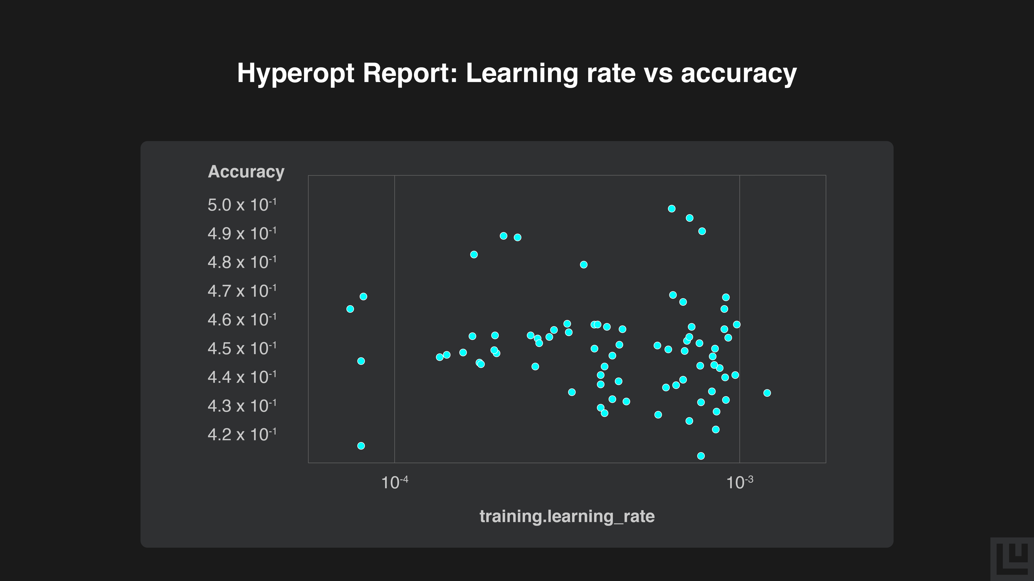
Our top three samples all had learning rates around 1/10³. Most of our other samples plateaued at around 46% - 47% accuracy.

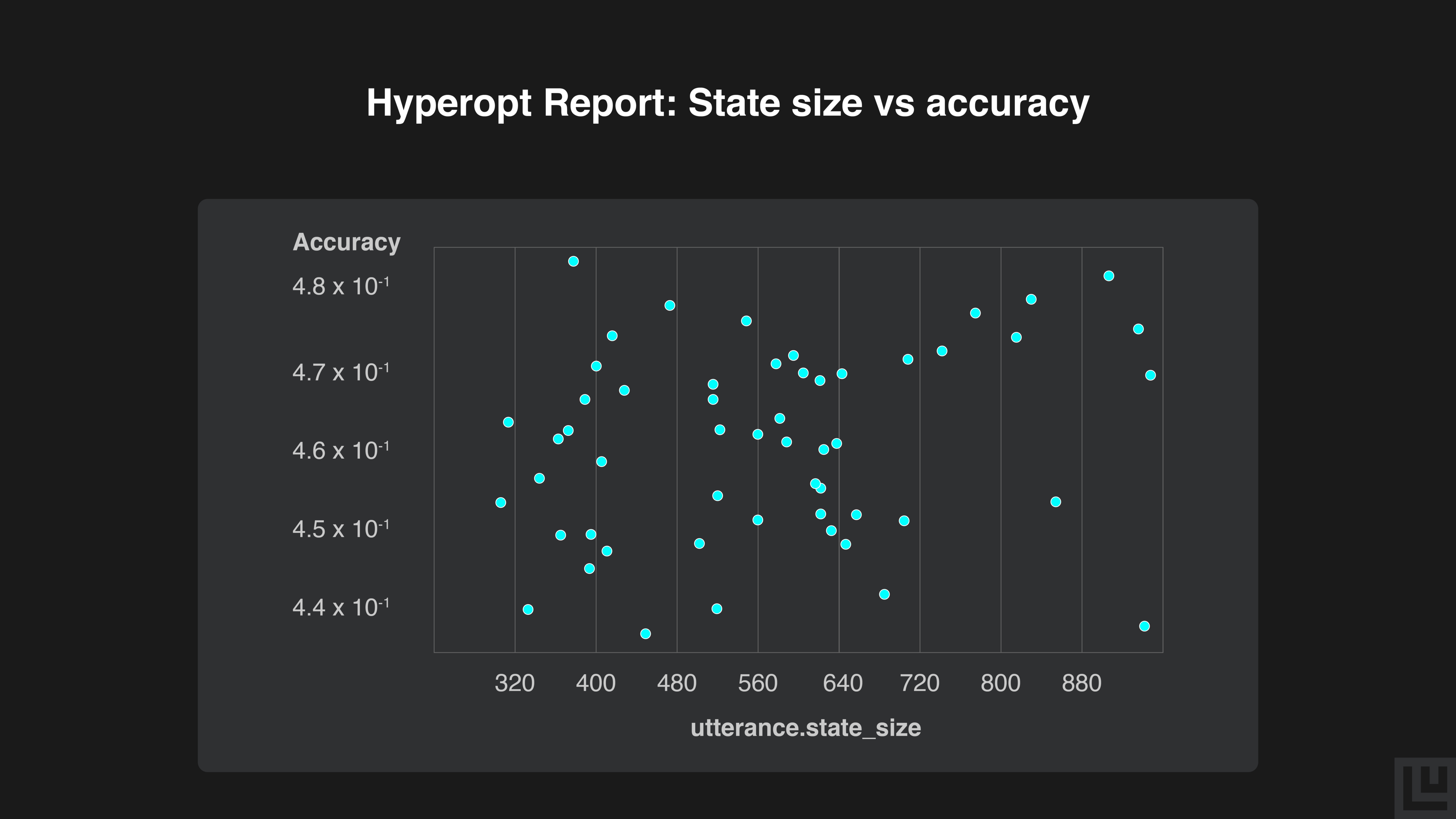
State sizes around the middle (600) have very consistent performance at around 45% - 47% accuracy, while state sizes closer to the edges (300 and 900) have a greater variance in results that produce some of our best and some of our worst samples.

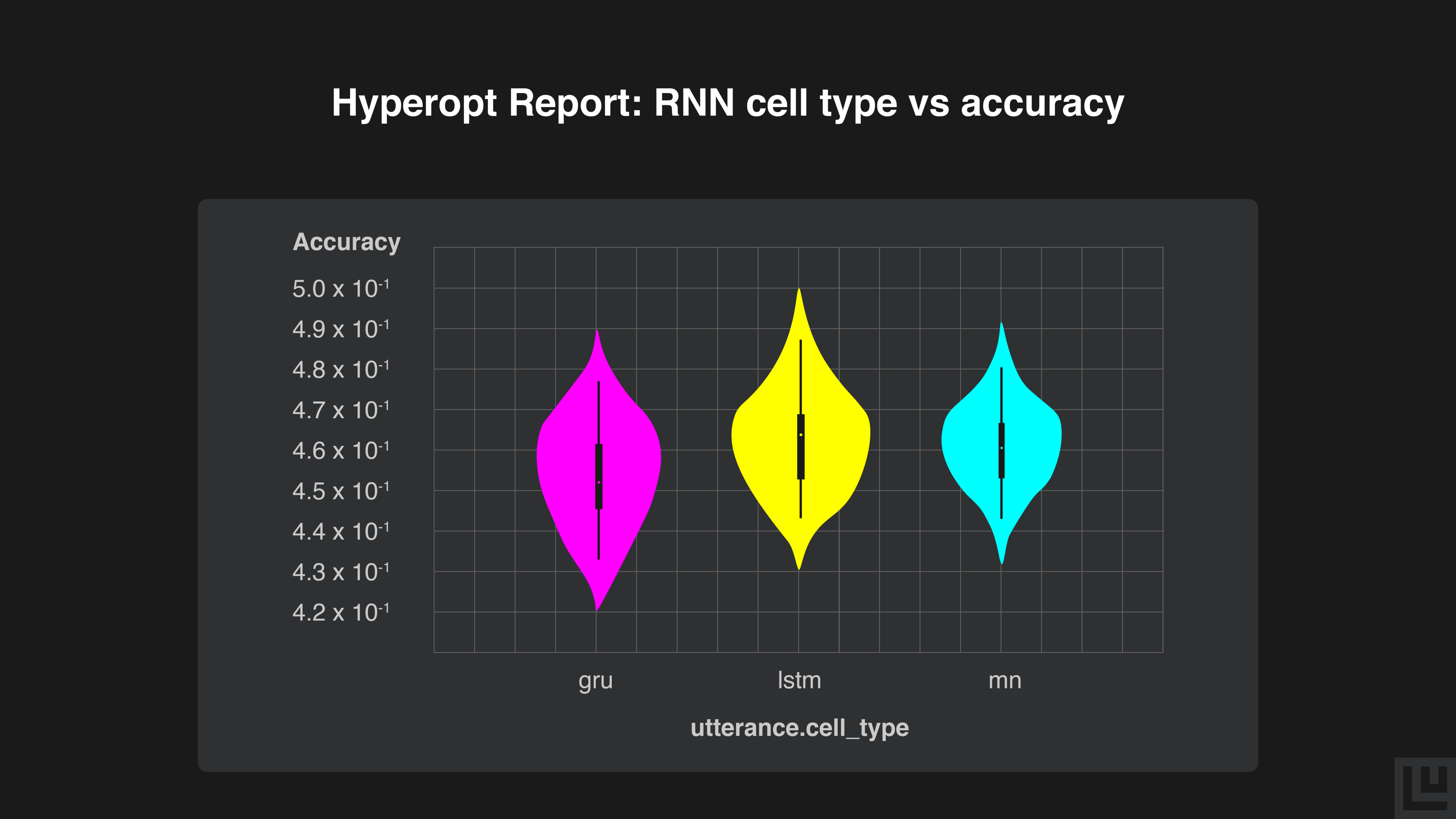
The LSTM cell has the best average performance as indicated by the white dot and the vertical black line, and also achieves the best performance. The RNN cell performs competitively, while the GRU performs worse.

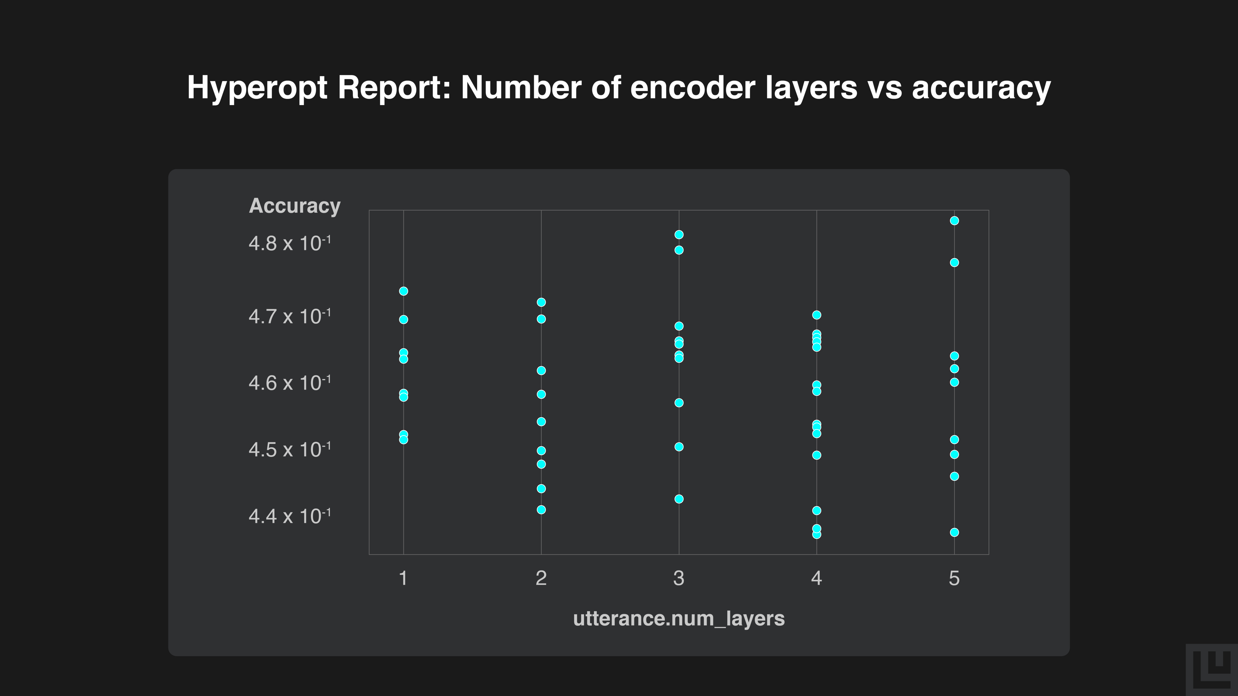
There doesn’t seem to be any obvious trends in the relationship between number of layers and accuracy, although the best performing samples have used 3 or 5 layers. It is possible that we would need more hyperparameter samples in order to observe a clear trend.

Hiplot

Ludwig also provides an integration with hiplot, which helps us visualize high-dimensional data through a parallel coordinate plot in an interactive webpage, where each hyperparameter has a vertical axis and a hyperparameter sample is plotted as a line passing through the axes, with a color dependent on the accuracy score.

from ludwig.visualize import hyperopt_hiplot_cli
hyperopt_hiplot_cli(
    'results/hyperopt_statistics.json',
    output_directory='./plots'
)

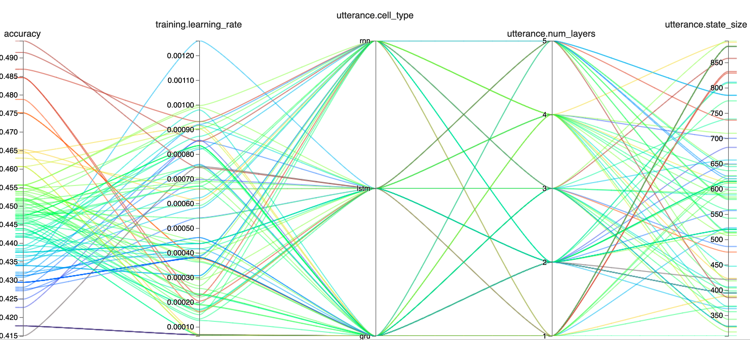
Screenshot of hiplot

From the hiplot we can see that the hyperparameter combination that gave us the best performance was:

• Learning rate: 0.0007445273631496333
• Encoder layers: 5
• Cell type: lstm
• State size: 385

We achieved an accuracy of 49.5% which is better than the 45.7% accuracy achieved in the original Recursive Deep Models for Semantic Compositionality Over a Sentiment Treebank paper by Socher et al. It is also slightly better than the 49.3% accuracy obtained by the Bi-LSTM model trained with default hyperparameters in Part 1.

Conclusion

In this post, we’ve seen how to perform hyperparameter optimization on a Recurrent Neural Network using Ludwig’s hyperopt module. Ludwig is a great toolkit for data scientists and machine learning engineers to use because it allows them to focus solely on the ML/DL aspect of their jobs. They can translate their intentions into a more user-friendly configuration file without having to worry about the code implementation.We encourage you to check out the documentation to learn more and to become engaged with the Ludwig open source community. We aim to make deep learning free and accessible to all. Also, follow Ludwig on Twitter to stay afloat with all news and developments. We hope you’ll join us.