A 3-part guide to go from importing dataset and implementing baseline models to working with BERT and doing Hyperparameter Optimization, all using only Ludwig.
You can follow along with the code through the Colab notebook.
Authors: Kanishk Kalra, Michael Zhu, Elias Castro Hernandez, and Piero Molino
Thanks to Debbie Yuen for the Images
If haven’t heard of Ludwig yet, then the first question that arises is What is Ludwig?
Ludwig is a user-friendly deep learning toolbox that allows users to train and test deep learning models on a variety of applications, including many natural language processing ones like sentiment analysis.
This article shows the ease with which production-ready models, from simple to the state-of-the-art, can be trained and tested in just a few lines of code using Ludwig and how to use Ludwig's visualization module to analyze them. All is done by simply defining inputs, outputs and few additional parameters without any need of pre-processing or implementing models and machine learning code from scratch.
Let’s quickly introduce the problem that we’d be working upon to demonstrate how one can use Ludwig to tackle it. We’ll be approaching one of the most common and popular tasks in Natural Language Processing (NLP), Sentiment Analysis. Sentiment Analysis is one of the tasks in NLP that involves classifying a piece of text with respect to the polarity of the sentiment it conveys. Usually, sentiment analysis datasets come either with binary labels indicating positive or negative sentiment or with more graded annotations. The dataset that we are going to use for this article is the well known Stanford Sentiment Treebank (SST).
SST is a sentence-level corpus of 10,662 labelled sentences created via a crowd-sourced effort to manually label the original Rotten Tomatoes Dataset (Pang & Lee 2005), which contains sentences from movie reviews with labels for every single phrase in each of the branches of the parse trees for all the sentences.
SST corpus comprises of both:
- SST-2 annotations — negative (0), neutral (1), and positive (2)
- SST-5 annotations — very negative (0), negative (1), neutral (2), positive (3), and very positive (4)
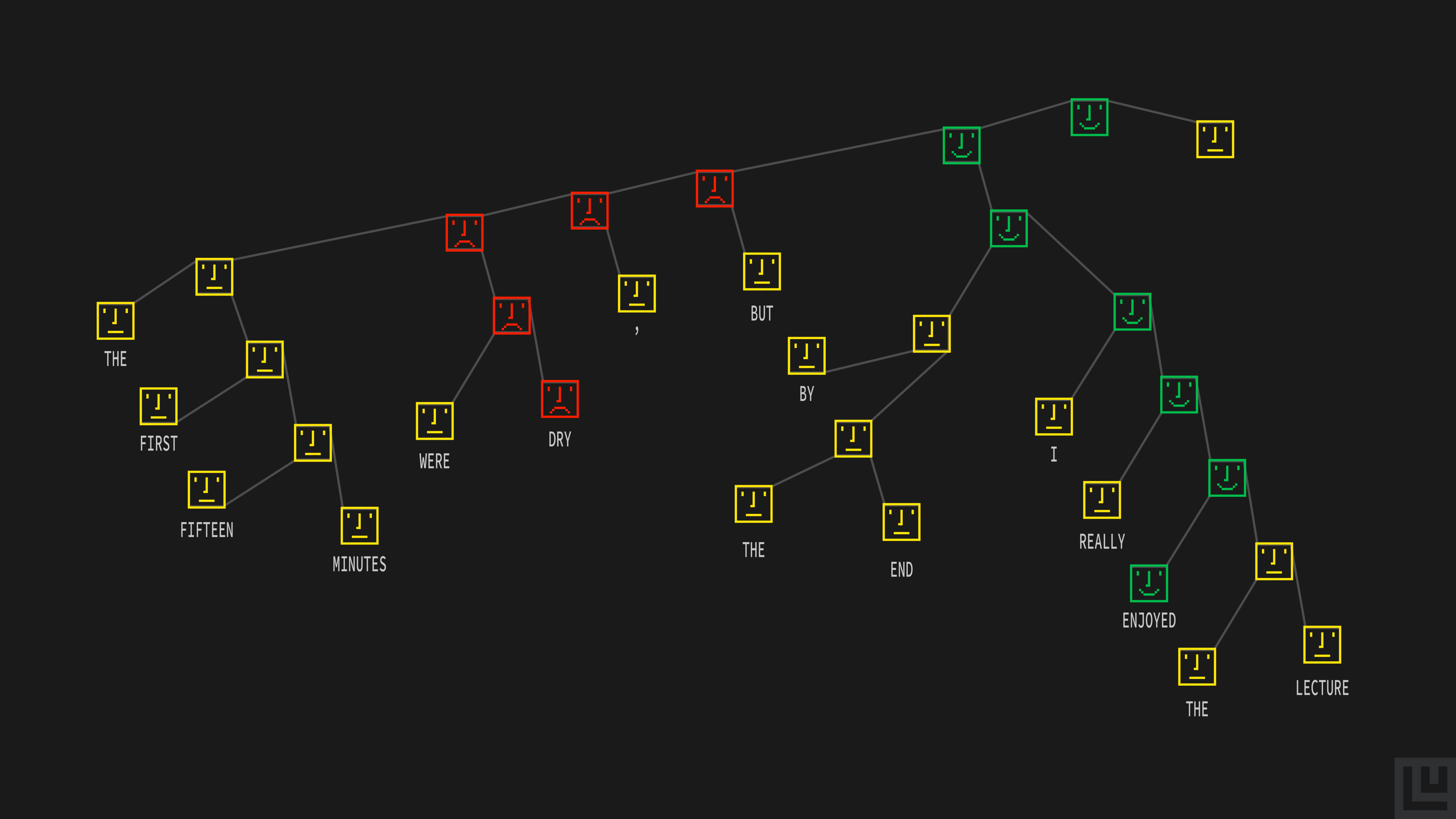
Parse Tree for a Simple Sentence adapted from Socher et al. (2013)
We will use just the phrases and their annotations, discarding the parse tree information.
Let’s start the setup by installing Ludwig using pip. As we are going to work with text and visualize our model performances, let’s also install the relevant subpackages.
$ pip install — quiet ludwig[text,viz]
Moving on to preparing our environment by importing some necessary packages:
import ludwig
from ludwig.api import LudwigModel
from ludwig.visualize import learning_curves, compare_performance, compare_classifiers_predictions
from ludwig.utils.data_utils import load_json
from ludwig.utils.nlp_utils import load_nlp_pipeline, process_text

# data and visualization
import numpy as np
import pandas as pd
from matplotlib import pyplot as plt
from wordcloud import WordCloud, STOPWORDS

# dataset utils
from torchtext import data
from torchtext import datasets

# auxiliary packages
import os
import yaml
import logging
import json
from tqdm.notebook import trange
Loading and minor preprocessing of the dataset
We’ll be using Torchtext to download the SST dataset.
We will be working on SST-5 which can be retrieved from torchtext.datasets.SST by setting fine_grained=Truebut you can choose to work with SST-2 as well by setting fine_grained=False.
# pick either SST-2 (False) or SST-5 (True)
fine_grained = True

if(fine_grained):
  # define SST-5 classes for sentiment labels
  idx2class = ['very negative', 'negative', 'neutral', 'positive', 'very positive']
  class2idx = {cls: idx for idx, cls in enumerate(idx2class)}
else:
  # define SST-2 classes for sentiment labels
  idx2class = ["negative", "neutral", "positive"]
  class2idx = {cls: idx for idx, cls in enumerate(idx2class)}

text_field = data.Field(sequential=False)
label_field = data.Field(sequential=False)  # False means no tokenization

# obtain pre-split data into training, validation and testing sets
train_split, val_split, test_split = datasets.SST.splits(
    text_field,
    label_field,
    fine_grained=fine_grained,
    train_subtrees=True  # use all subtrees in the training set
)
Ludwig allows a variety of formats to be processed, but for simplicity let’s transform the SST-5 dataset into a Pandas DataFrame.
# obtain texts and labels from the training set
x_train = []
y_train = []
for i in trange(len(train_split), desc='Train'):
    x_train.append(vars(train_split[i])["text"])
    y_train.append(class2idx[vars(train_split[i])["label"]])

# obtain texts and labels from the validation set
x_val = []
y_val = []
for i in trange(len(val_split), desc='Validation'):
    x_val.append(vars(val_split[i])["text"])
    y_val.append(class2idx[vars(val_split[i])["label"]])

# obtain texts and labels from the test set
x_test = []
y_test = []
for i in trange(len(test_split), desc='Test'):
    x_test.append(vars(test_split[i])["text"])
    y_test.append(class2idx[vars(test_split[i])["label"]])

# create three separate dataframes
train_data = pd.DataFrame({"text": x_train, "label": y_train})
validation_data = pd.DataFrame({"text": x_val, "label": y_val})
test_data = pd.DataFrame({"text": x_test, "label": y_test})
Exploratory data analysis
After transformation into DataFrames, Now let’s inspect it, both to get a flavor of its content and to figure out how balanced it is.
# preview sample of data with class labels
labels = [idx2class[int(id)] for id in train_data['label']]

train_data_preview = train_data.drop(columns='label').assign(class_id=train_data['label'], class_label=labels)

train_data_preview.head()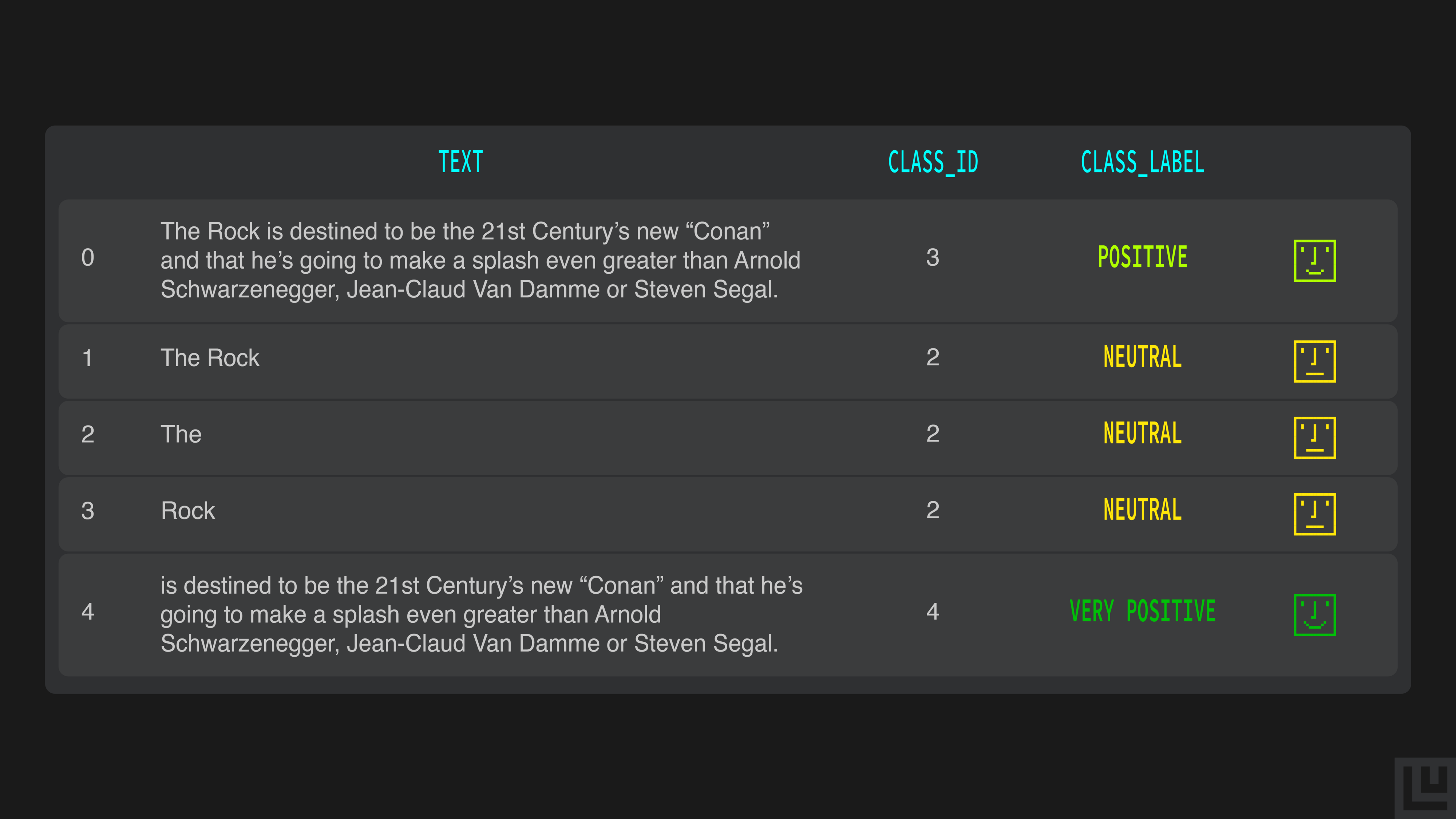
Let’s also look at the class distribution of the training set to get an intuition of its balance.
# plotting look
plt.style.use('ggplot')

fig, ax = plt.subplots()

if fine_grained:
  ax.set_title(f'Distribution of sentiment labels in the SST-5 training set')
  ax = train_data['label'].value_counts(sort=False).plot(kind='barh', color=['red', 'coral', 'grey', 'lime', 'green'])
else:
  ax.set_title(f'Distribution of sentiment labels in the SST-2 training set')
  ax = train_data['label'].value_counts(sort=False).plot(kind='barh', color=['red','green'])

# axes info
ax.set_xlabel('Samples in the training set')
ax.set_ylabel('Labels')
ax.set_yticklabels(tuple(idx2class))
ax.grid(True)
plt.show()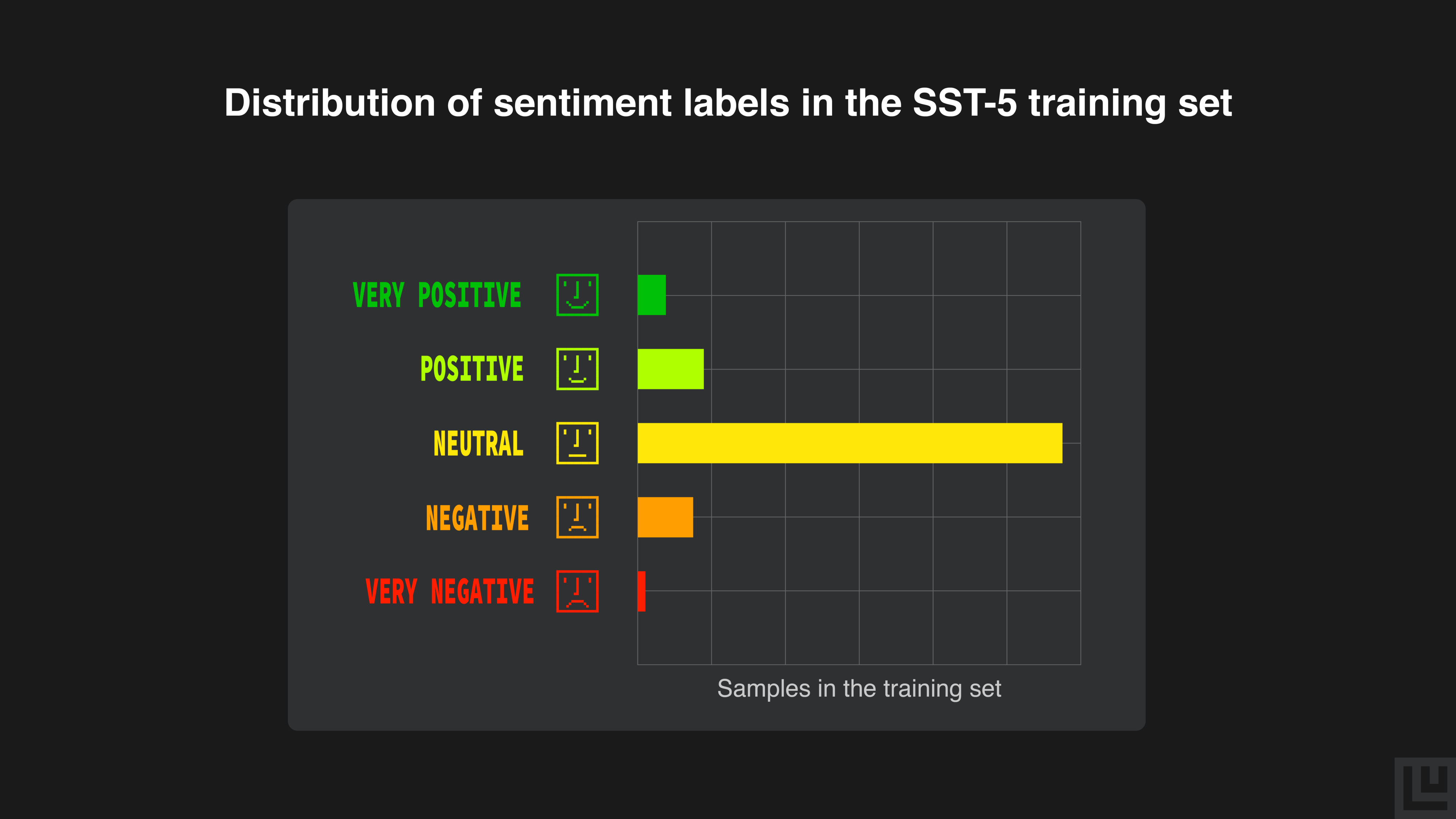
The plot shows how the neutral class is by far the most frequent in the dataset. The reason for this is that we are using all phrases in the reviews and many of them are neutral despite being part of more polarized reviews.
A word cloud can moreover give us an overview of the content of the dataset by showing the words appearing in it most frequently.
processed_train_data = process_text(' '.join(train_data['text']),
                                    load_nlp_pipeline('en'),
                                    filter_punctuation=True,
                                    filter_stopwords=True)

wordcloud = WordCloud(background_color='black', collocations=False,
                      stopwords=STOPWORDS).generate(' '.join(processed_train_data))

plt.figure(figsize=(8,8))
plt.imshow(wordcloud.recolor(color_func=lambda *args, **kwargs:'white'), interpolation='bilinear')
plt.axis('off')
plt.show()
Model Selection — Baseline to SOTA
In order to obtain a model that predicts the sentiment of the movie reviews in SST, we need to train a multi-class text classifier. We are going to train a few models to know how well they perform on the sentiment analysis task using this dataset and compare them.
We will be exploring the following models:
I. Parallel CNN, similar to a WordCNN, one of the first successful deep learning models applied to language tasks,
II. Bidirectional LSTM and finally,
III. A pre-trained BERT model.
We chose these models because they are different in terms of complexity and computational requirements. Ludwig provides more models architectures to play with, and even more can be added very easily.
In the first two models we are going to use pre-trained word embeddings, so let’s quickly introduce them.
What are pre-trained embeddings and why are they useful?
Word vectors, or embeddings, are a way of representing words with a fixed-size dense vector. These fixed-size vectors are learned to represent words based on the contexts in which they appear in a reference corpus, which is usually huge in size. They can be trained using different algorithms such as word2vec or GloVe.
When used as the first layer of neural networks, pre-trained embeddings have been shown to provide a boost in sentiment analysis performance, as they transfer information learned on bigger corpora.
We are going to use GloVe embeddings, so let’s download them:
# extracting the GloVe embeddings takes ~7 minutes with a decent internet connection

# download pre-trained embeddings GloVe
!wget http://downloads.cs.stanford.edu/nlp/data/glove.6B.zip

# unzip to glove dir
!unzip /content/glove.6B.zip -d glove/
I. Parallel CNN
The Parallel CNN encoder is a more general version of the WordCNN model presented in Convolutional Neural Networks for Sentence Classification by Yoon Kim. The paper proposes to use convolutional layers with filters of different sizes in parallel to perform sentence classification and showed good results on sentence classification tasks like sentiment analysis and question classification. It was also among the first papers to use pre-trained embeddings, which has then become a common practice.
For a detailed explanation of CNNs refer to this article or the explanation from Stanford CS231. Also, for CNNs in context to text refer to this blog or A Primer on Neural Network Models for NLP, Section 9 by Yoav Goldberg.
Building Parallel CNN Using Ludwig
To build a Ludwig model, we first need to define a configuration.
The configuration contains information about the inputs to the models, its outputs, training and preprocessing parameters and hyperparameters to optimize. Given a configuration, Ludwig assembles a model depending on the data type of inputs and outputs.
Since our dataset contains an input text and an output category, our configuration will contain one input feature of type text and one output feature of type category.
When defining input features, we have to provide a list of dictionaries, one for each feature. Each dictionary should contain a name (the name of the column in the DataFrame that contains it) and a type, in our case text. We can also specify several additional optional parameters:
- the level of representation (e.g. words or characters —
'level': 'word'). - the type of neural network architecture we want to use (
'encoder': 'parallel_cnn') and its parameters (number of filters with their sizes, number of fully-connected layers with their sizes). - the word embeddings to load, their size, the vocabulary to use.
Similarly, we can specify several training parameters in the training section as:
- learning rate or if to use decay or not -
'learning_rate': 0.001,'decay': True. - the output feature to use for validation —
'validation_field': 'label'. - the metric to use for validation and early stopping —
'validation_metric': 'accuracy'.
Though we have briefly looked over the list of configurable parameters, there are a lot more. Refer to the User Guide to get a complete list of them. Additionally, check the Examples page for examples of simple configurations for several machine learning tasks other than text classification.
config = {
    'input_features': [{
        'name': 'text',
        'type': 'text',
        'level': 'word',
        'encoder': 'parallel_cnn',
        'pretrained_embeddings': '/content/glove/glove.6B.300d.txt',
        'embedding_size': 300,
        'preprocessing': { 'word_vocab_file': '/content/glove/glove.6B.300d.txt' }
    }],
    'output_features': [{'name': 'label', 'type': 'category'}],
    'training': {
        'decay': True,
        'learning_rate': 0.001,
        'validation_field': 'label',
        'validation_metric': 'accuracy'
    }
}
After defining our configuration, we just need to create a LudwigModel instance and train it using the DataFrames previously obtained.
print("Instantiating LudwigModel...")
parallel_cnn = LudwigModel(config, logging_level=logging.DEBUG)

print("Training Model...")
train_stats_parallel_cnn, _, _ = parallel_cnn.train(
    training_set=train_data,
    validation_set=validation_data,
    test_set=test_data,
    model_name='parallel_cnn',
    skip_save_processed_input=True
)
Visualizing and Interpreting Parallel CNN’s Results
We successfully trained a Parallel CNN using Ludwig and the training statistics were returned in the train_stats_parallel_cnn variable.
Let’s visualize these statistics to better understand the training process. Ludwig makes it easy to visualize the learning curves with different metrics (the loss, the accuracy and hits at k) by calling the learning_curves function.
# visualizing the training results
learning_curves(train_stats_parallel_cnn, output_feature_name='label', model_names='parallel_cnn')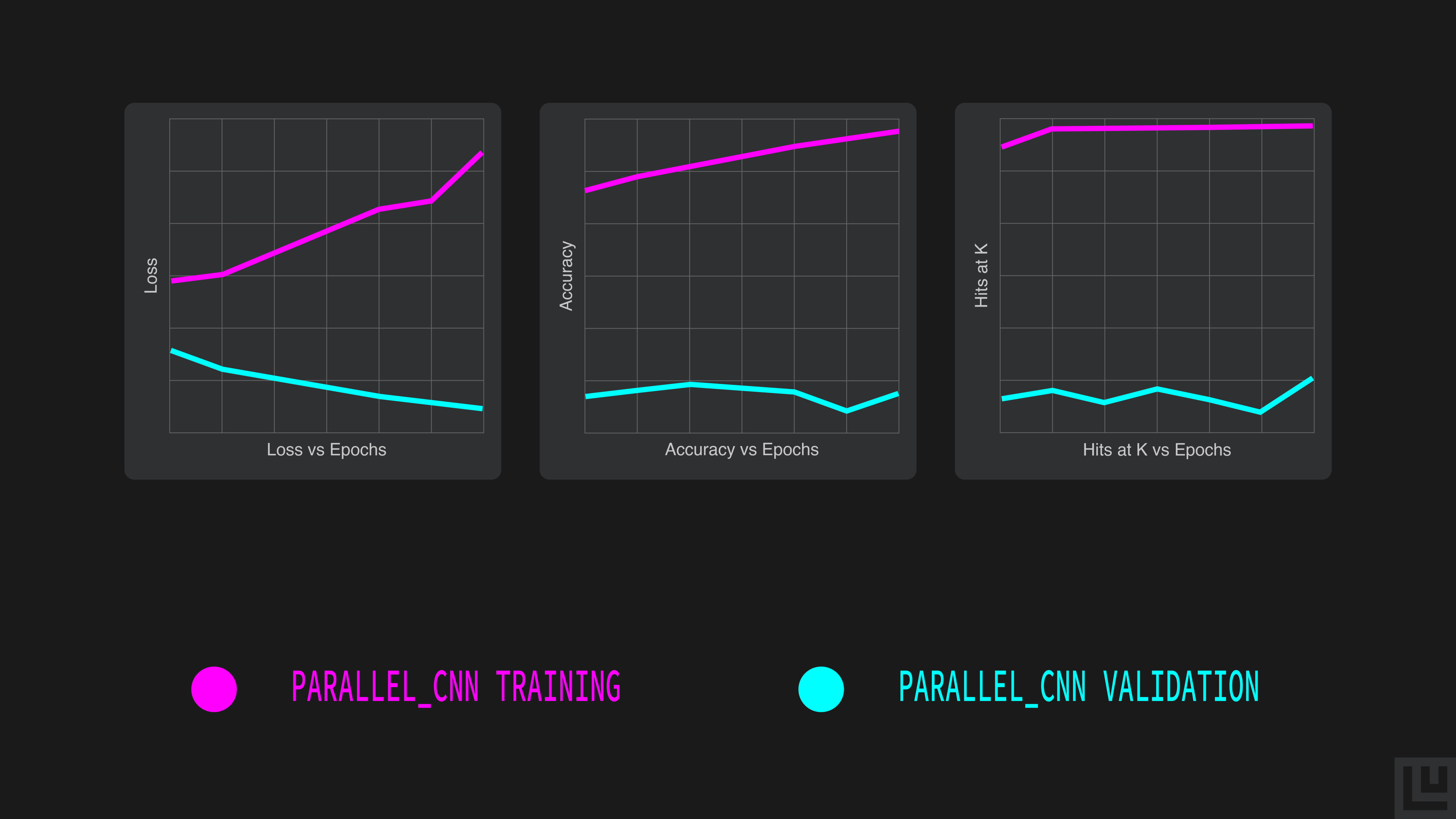
The above graphs showing the learning curves with different metrics (the loss itself, the accuracy, and hits at k) demonstrate how the model achieves its maximum performance on the validation set (validation accuracy of 48.7% at epoch 4) and plateauing thereafter, although most of the training improvement was already obtained in the first two epochs.
We do observe a significant gap between the training and validation curves. This is indicative of the model underfitting. Hence, we must try some other model which captures more variance.
II. Bidirectional LSTM (Long Short Term Memory)
Parallel CNNs perform well on NLP tasks and have the advantage of being fast to train, but may have problems dealing with language compositionality and long dependencies, as suggested in a paper by Yi Yang.
By comparison, Recurrent Neural Networks (RNN) provides an architecture that helps with language compositionality as well as long term dependencies in language — with its recurrent structure, which is well suited for sequences. Though RNNs provide flexibility in processing variable sized inputs, they are susceptible to the vanishing gradient problem which limits the length of the dependencies.
Long Short Term Memory (LSTM) is a type of RNN that uses a different cell as the operation to apply to each time step. This modified cell, through the use of a memory that is written to and read from, mitigates the vanishing gradient problem.
In our model, we make the LSTM bidirectional by having a separate layer for each direction (left→right and right→left) and then concatenating their outputs.
For more details on RNNs refer to the paper by Paul Rodriguez, Janet Wiles & Jeffrey L. Elman and for LSTMs refer to the paper by Hochreiter and Schmidhuber.
Building Bidirectional LSTM Using Ludwig
Just as we defined a configuration for Parallel CNN, we follow the exact same pattern to define a configuration for a bidirectional LSTM but, changing and adding a few parameters to input_features. We change the encoder to RNN ('encoder': 'rnn') with an LSTM cell ('cell_type': 'lstm'), that is applied in both directions (
'bidirectional': True) and keep the other parameters the same.config = {
'input_features': [{
'name': 'text',
'type': 'text',
'level': 'word',
'encoder': 'rnn',
'cell_type': 'lstm',
'bidirectional': True,
'pretrained_embeddings': '/content/glove/glove.6B.300d.txt',
'embedding_size': 300,
'preprocessing': {'word_vocab_file': '/content/glove/glove.6B.300d.txt'}
}],
'output_features': [{'name': 'label', 'type': 'category'}],
'training': {
'decay': True,
'learning_rate': 0.001,
'validation_field': 'label',
'validation_metric': 'accuracy'
}
}
print("Instantiating LudwigModel...")
bi_lstm = LudwigModel(config, logging_level=logging.DEBUG)
print("Training Model...")
train_stats_bi_lstm, _, _ = bi_lstm.train(
training_set=train_data,
validation_set=validation_data,
test_set=test_data,
model_name='bi_lstm',
skip_save_processed_input=True
)Visualizing and Interpreting Bidirectional LSTM’s Results
Like we did for the ParallelCNN, let’s visualize the learning curves.
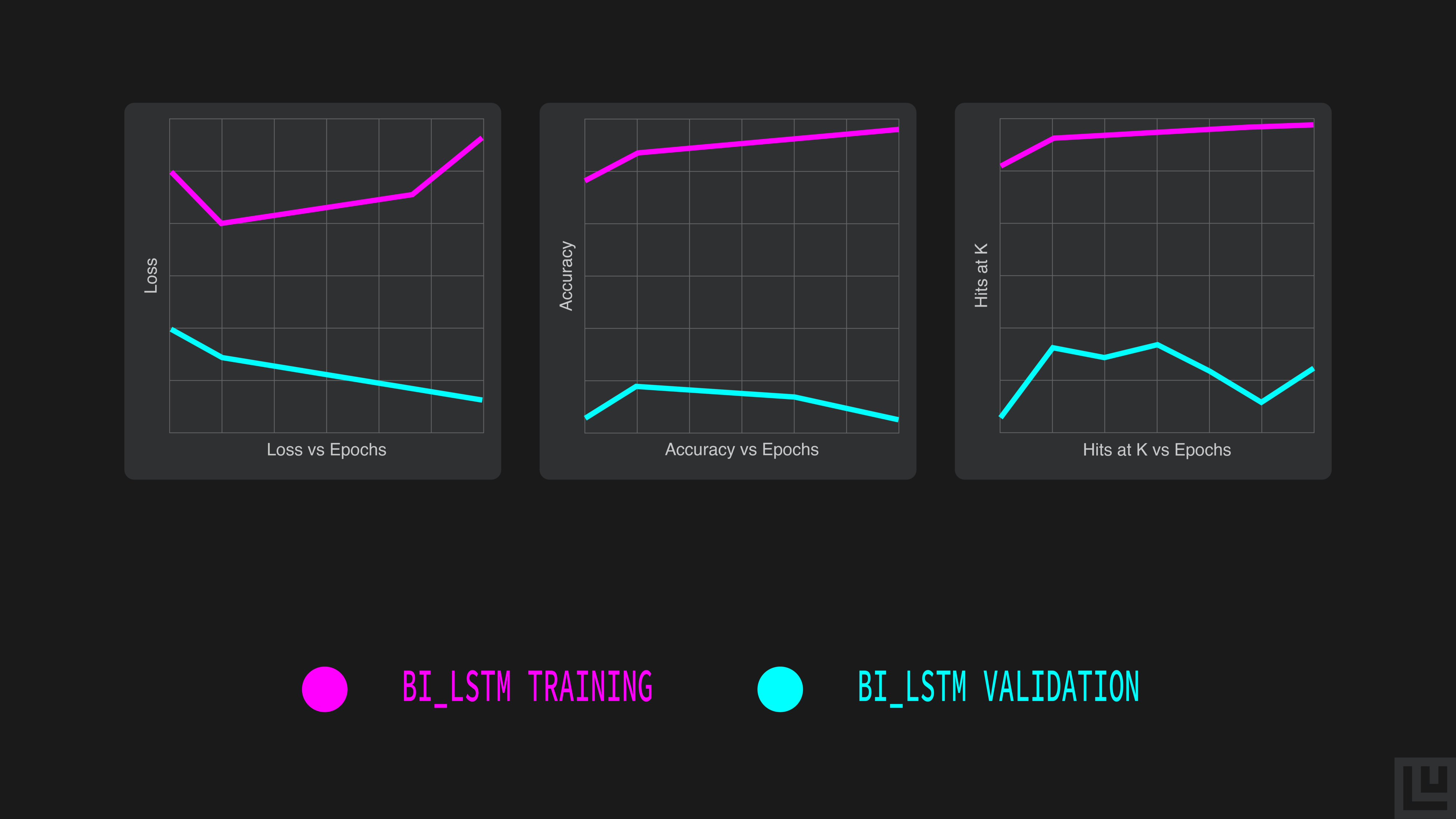
Just a glance over the Bi-LSTM’s learning curves helps us identify that the model achieved a maximum validation accuracy of 49.3% on epoch 2.We observe that the performance achieved by the Bi-LSTM is slightly higher than the Parallel CNN. Depending on our deployment constraints, the added computation cost of the Bi-LSTM may or may not be worth the improved performance. There is still scope for improvement that leads us to the last model in our list, BERT.
Check out Part 2 of the series where we discuss BERT and compare all the models we trained. Want to know how you can easily optimize the hyperparameters of your Ludwig models? Skip to Part 3 of the series where we discuss hyperparameter optimization.
We encourage you to check out the documentation to learn more and to become engaged with the Ludwig open source community. We aim to make deep learning free and accessible to all. Also, follow Ludwig on Twitter to stay afloat with all news and developments. We hope you’ll join us.


