Introduction

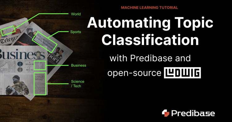
Topic classification is an important machine learning use case for businesses that deal with large volumes of unstructured text data, but building state-of-the-art NLP pipelines can be a challenge. Let’s go through the simple process of building an end-to-end topic classification model using Predibase, the low-code declarative ML platform, and the open-source project Ludwig. In 5 easy steps, this tutorial will show you how to connect data, build various models in a declarative way, and query your models with SQL-like commands using PQL (Predictive Query Language).

Automating Topic Classification with ML 

Topic classification can help you improve efficiency across a wide set of business applications. By automating the process of categorizing documents, you can reduce the time and effort required to manually sort and label documents, articles, customer feedback and more. You can use topic classification models for many use cases like labeling customer support tickets, tagging content, detecting spam/toxic messages, and sorting internal files.

For this tutorial, we are going to use the AG News dataset hosted on Kaggle. AG is a collection of more than 1 million news articles. The AG's news topic classification dataset is constructed by choosing the four largest classes from the original corpus. Each class contains 30,000 training samples and the total number of training samples is 120,000. This dataset includes two features: “titles” and “descriptions”. The four topic classes in the target variable are “world”, “business”, “sci_tech”, and “sports”. The original dataset includes a numerical index, and to improve comprehension of the model later on, a column called “Class” has been added to map the class index to their meanings.

The ML task here is to classify the news into distinct topics based on unstructured text features: news titles and descriptions. We’ll show you how to build an end-to-end NLP pipeline for this task in 5 easy steps and then iterate on the model for better performance. Let’s get started!

Step 1: Connecting Text Data

Predibase allows you to instantly connect to both your local directory and cloud data sources, pulling in all your data - including tabular, text, images, audio, and more - wherever it may live. For today’s example, we are going to upload the dataset from a local directory by clicking the “File” icon.

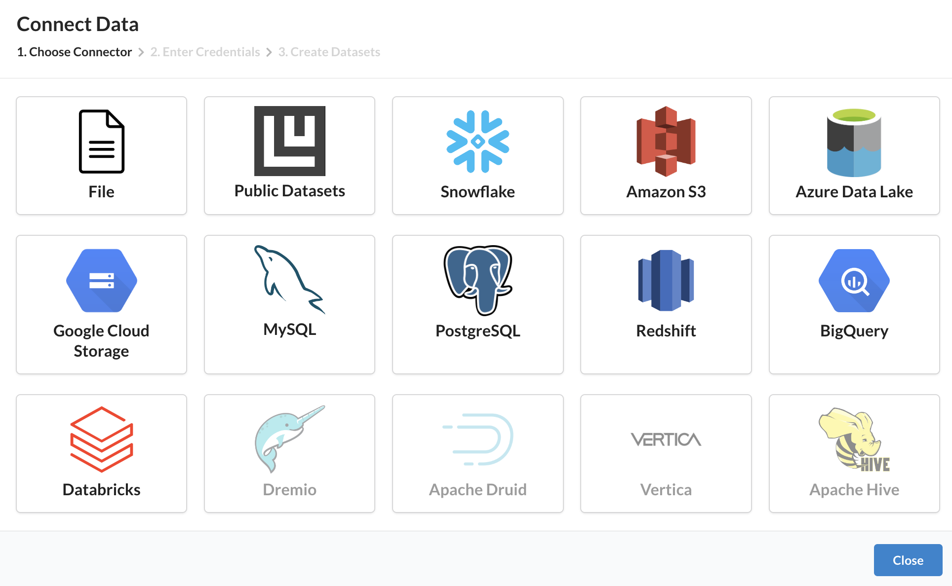
Instantly connect to all of your data - including tabular, text, images, audio, and more - wherever it may live.

Step 2: Building our first topic classification model

Before we build our first model, let me explain how Predibase works. Predibase is the first platform to take a low-code declarative approach to machine learning. Instead of writing thousands of lines of code, you can build state-of-the-art models with concise but flexible configurations. Declarative ML systems are adopted in leading tech companies. Apple, Meta, and Uber have all developed internal declarative ML frameworks. 

The algorithms used in Predibase are based on the open-source Ludwig framework originally developed at Uber (8,800+ stars on GitHub). With Ludwig, all you have to do is specify your input and output features in a configuration-driven manner – in this case, YAML –  to start to train your baselines. Predibase simplifies this modeling process even further, reducing the process to arrive at a trained model to just a few clicks. 

Want to see declarative ML in action? Let’s train our first model to see how it works.

If you don’t know what kind of config is best for your first model, Predibase will suggest one based on the types of datasets after you select “Basic defaults”.

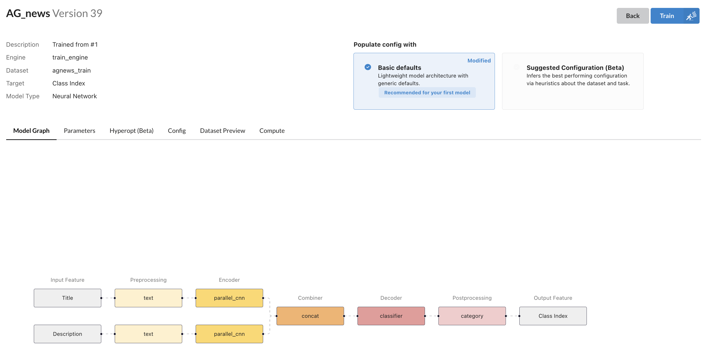
Predibase automatically generates a visualization of the suggested model architecture.

At Predibase, we visualize the model architecture for you. For example, you can see that we use parellel_cnn as an encoder for input features, and they later go through the concat combiner. The concat combiner assumes all outputs from encoders. It concatenates and then optionally passes the concatenated tensor through a stack of fully connected layers. If you’re curious to learn more about the Encoder-Combiner-Decoder (ECD) architecture, you can visit the docs to read more about Ludwig’s architecture.

Based on the data, Predibase suggests this config to get your first trained model:

input_features:
  - name: Title
    type: text
    column: Title
  - name: Description
    type: text
    column: Description
output_features:
  - name: Class
    type: category
    column: Class

Result

You can simply click train to kick off model training. When it’s ready, you will have access to various model performance metrics as well as the hyperparameters used for training.  Since this is a dataset with balanced classes, let’s use accuracy and ROC to evaluate the model.  For our first model, the test accuracy is 0.9158, and the ROC is 0.9857. This is the power of Ludwig and Predibase: great results out of the box with the ability to easily fine-tune to improve even further as desired. 

Let’s look at the learning curve. It looks like the loss of the validation set and test set didn’t converge, and it’s overfitted. Let’s see if we can iterate the model to make it converge and improve the model performance.

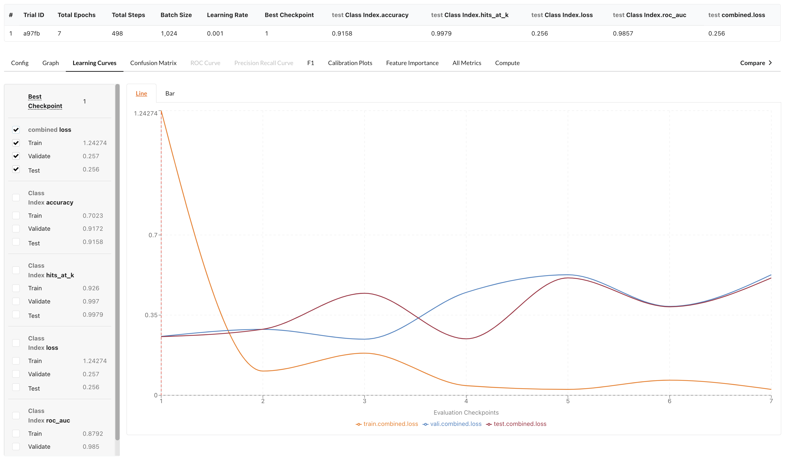
Predibase provides visualizations on model performance. In this case, the learning curve shows overfitting.

Step 3: Exploring suggested models

In the early stage of model development, it’s helpful to try a few different models and see what works well. With Predibase, you don’t need to manually set up those experiments, you can simply select “Explore suggested models”. For text datasets, this will give you 6 models including the default ECD model, pre-trained 2 BERT models, and a few other deep learning models.

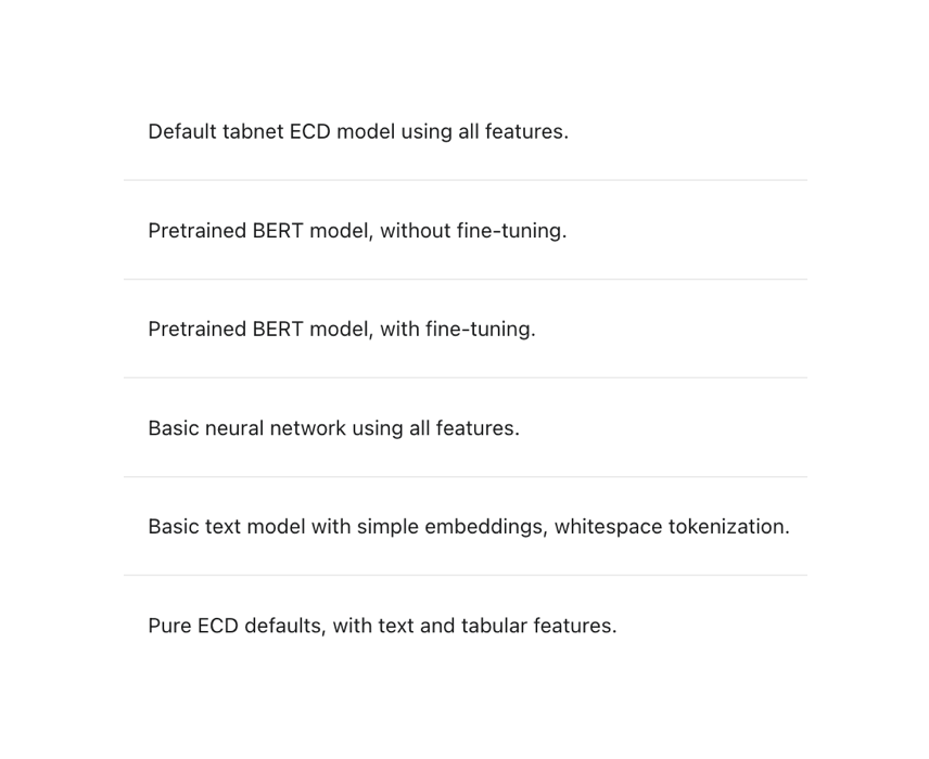
The Explore Suggested Models button provides a series of model architectures that make it easy to rapidly experiment with different model parameters like BERT for text encoding.

If you are not familiar with the ECD and BERT models, let me quickly explain.  

Ludwig’s core modeling architecture is referred to as ECD (encoder-combiner-decoder). Multiple input features are encoded and fed through the Combiner model that operates on encoded inputs to combine them. On the output side, the combiner model's outputs are fed to decoders for each output feature for predictions and post-processing. Learn more about Ludwig's architecture.

When visualized, the ECD architecture looks like a butterfly and sometimes we refer to it as the “butterfly architecture”.

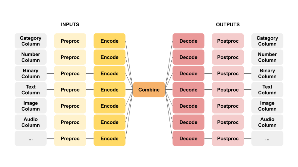
The ECD architecture supports many different machine learning use cases in a single unified architecture.

Ludwig also provides pre-trained models like GPT, ELECTRA, RoBERTa and BERT. The BERT model is considered state-of-the-art for language understanding that utilizes the Transformer architecture. BERT is a collection of models that consist of a deep stack of transformer layers that employ self-attention. By fine-tuning the pre-trained BERT models on specific datasets, we can achieve close to state-of-the-art performance in various token-level and sentence-level tasks. You can read more about BERT here.

Don’t worry if you don’t know the details of architectures of the models we use, we make it easy for you to run experiments on Predibase. Let’s kickstart the set of suggested models and see which one performs the best!

Result

After all 6 models have finished training, we found that the pre-trained BERT model with fine-tuning performs the best with an accuracy of 0.94 and ROC of 0.99. This is the config suggested by Predibase:

input_features:
  - name: Title
    type: text
    column: Title
  - name: Description
    type: text
    column: Description
output_features:
  - name: Class Index
    type: category
    column: Class Index
trainer:
  epochs: 5
  optimizer:
    type: adamw
  batch_size: auto
  learning_rate: 0.00001
  use_mixed_precision: true
  learning_rate_scheduler:
    decay: linear
    warmup_fraction: 0.2
defaults:
  text:
    encoder:
      type: bert
      trainable: true

Let’s look at the learning curve again. It looks like the loss of validation and test set did start converging this time, however, it’s still overfitted.

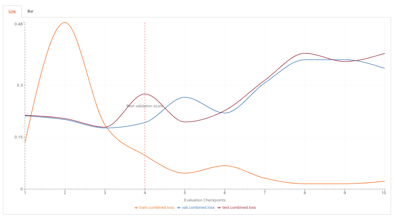
The learning curves shows that our model is still overfitting.

Let’s iterate the model and see if we can overcome overfitting.

Step 4: Diagnose and fix the model

It looks like the learning curve above has a few spikes, and it could indicate that the learning rate is too big. Let’s reduce the learning rate with the same config of the pre-trained BERT model.

All you need to do is to create a new model based on the existing one, and in the model config page, enter the learning rate as 0.000001.

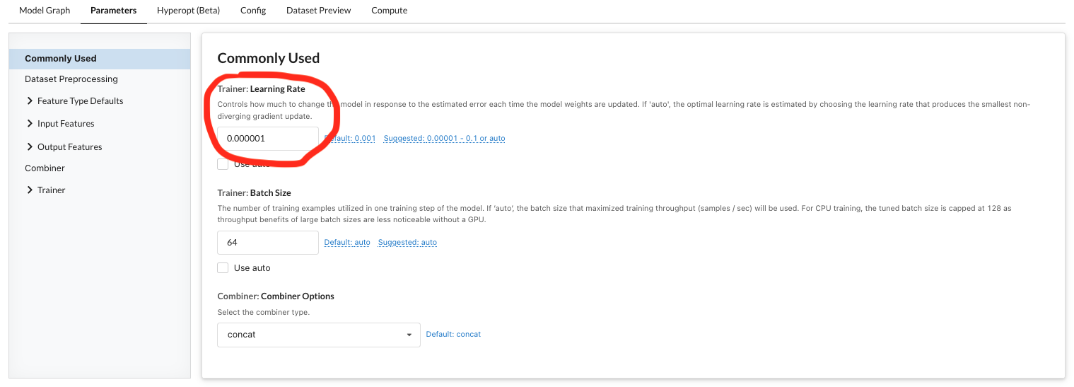
Changing the learning rate to help address overfitting.

We also want to train the model for longer this time as the learning rate is smaller, we set the epoch number to 20 instead of 5. Let’s kick off a model iteration with these new parameters!

Final Model Result

Finally, the model converged and we drastically reduced overfitting by reducing the learning rate and increasing the epochs. The accuracy on test data is 0.9309 and ROC is 0.9904. 

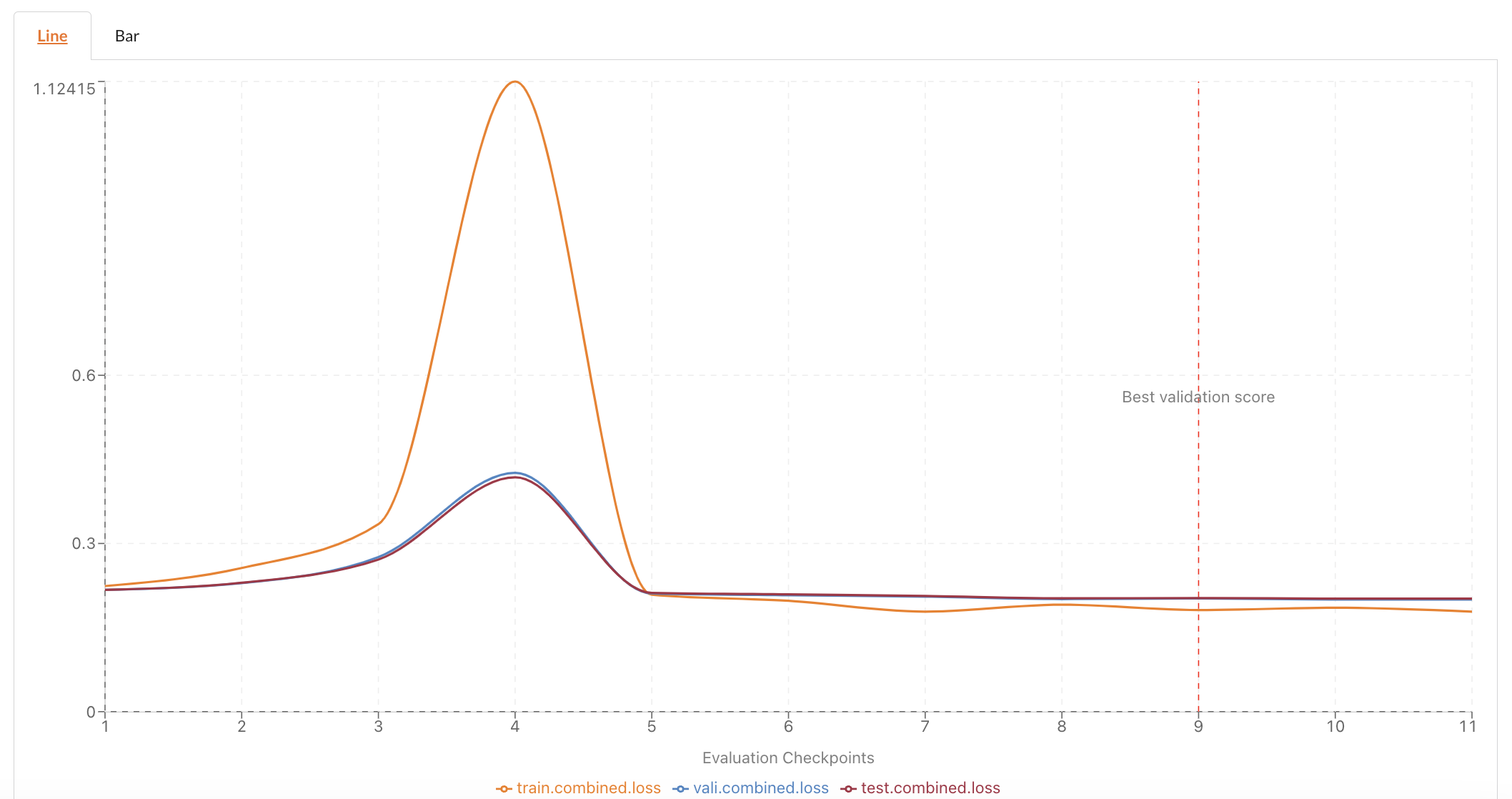
The learning curve for our updated model shows that our changes drastically reduced overfitting.

Model Deep Dives

To understand more about the model, you may want to investigate the model's performance for a few examples. In this case, we can utilize PQL (Predictive Query Language) to do this task. 

The syntax of PQL is very similar to SQL and you can use the query below to see what category the model predicts the data point into, and you get another column with an explanation where you can click into it.

PREDICT class WITH EXPLANATION
USING AG_news VERSION 33
GIVEN SELECT class,title, description FROM agnews_sanitized
LIMIT 5

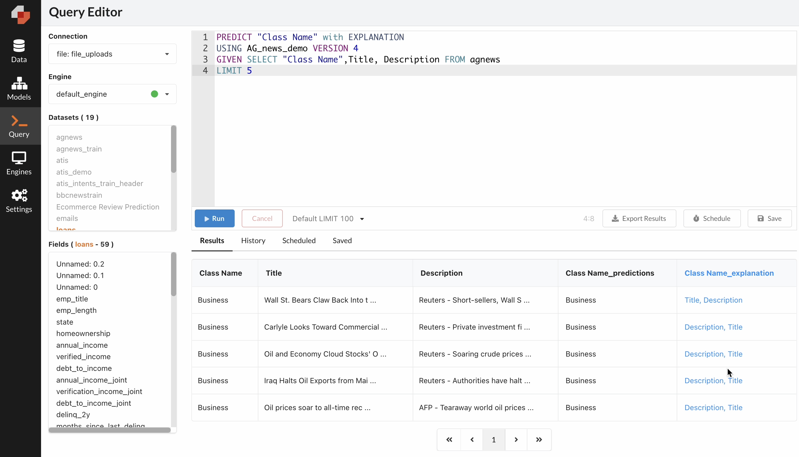
The Predictive Query Language Editor (PQL) enables us to explore the explanations of our predictions with simple SQL-like commands.

When you click into the explanation column and select “Text Explanation” to view text token-level explanations for the input text features. You’ll find the green tokens are evidence for the selected class and the red tokens are evidence against the class. In this example, the words “economy”, “stock”, “worries” helped the model predict this example into “Business” category. This helps you form assumptions on why the model performs well or not well on certain datasets and you can iterate the model further.

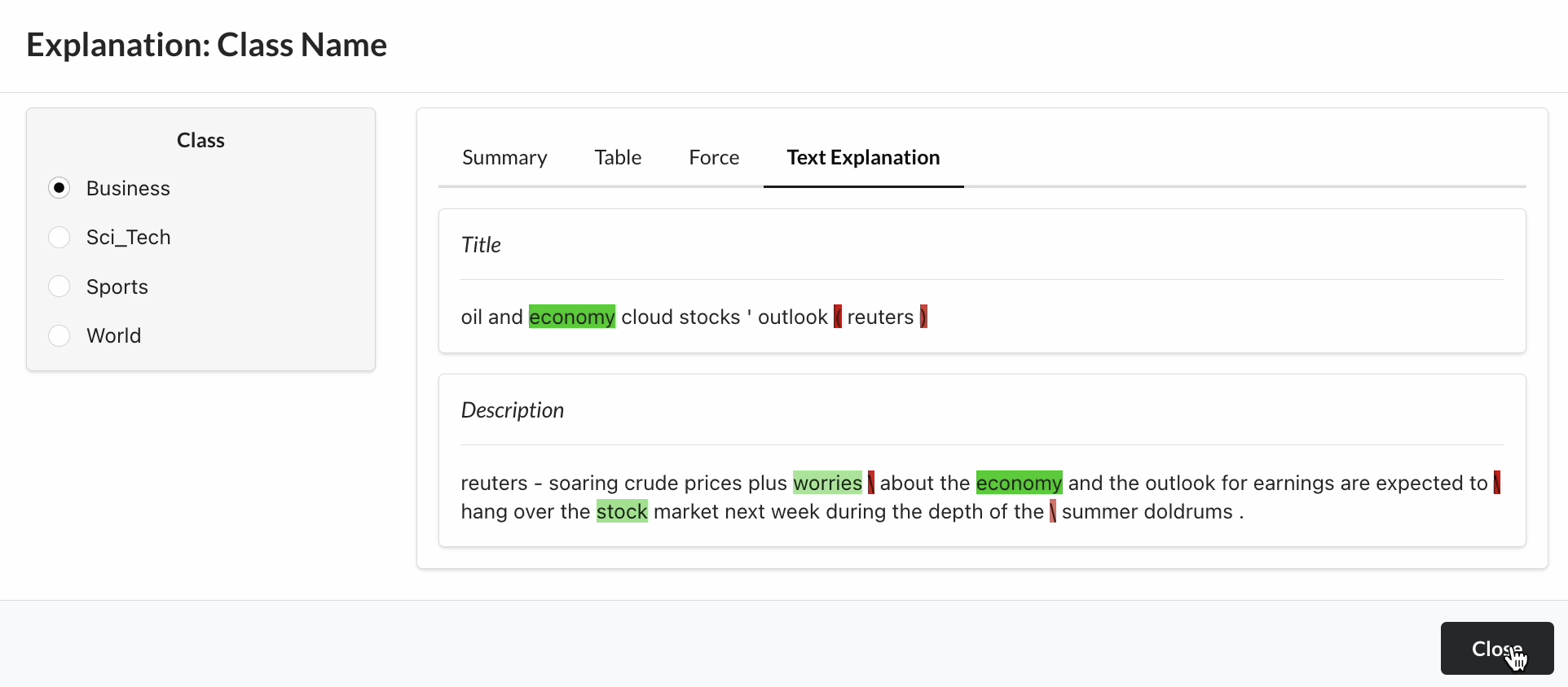
Visualizations provide token-level explanations to help us understand which text features had the greatest impact on our individual predictions.

Step 5: Deploy into production

Now that  we are satisfied with the model's performance, we can deploy it for production by clicking on the "deploy" button in the specific version of the model into production. 

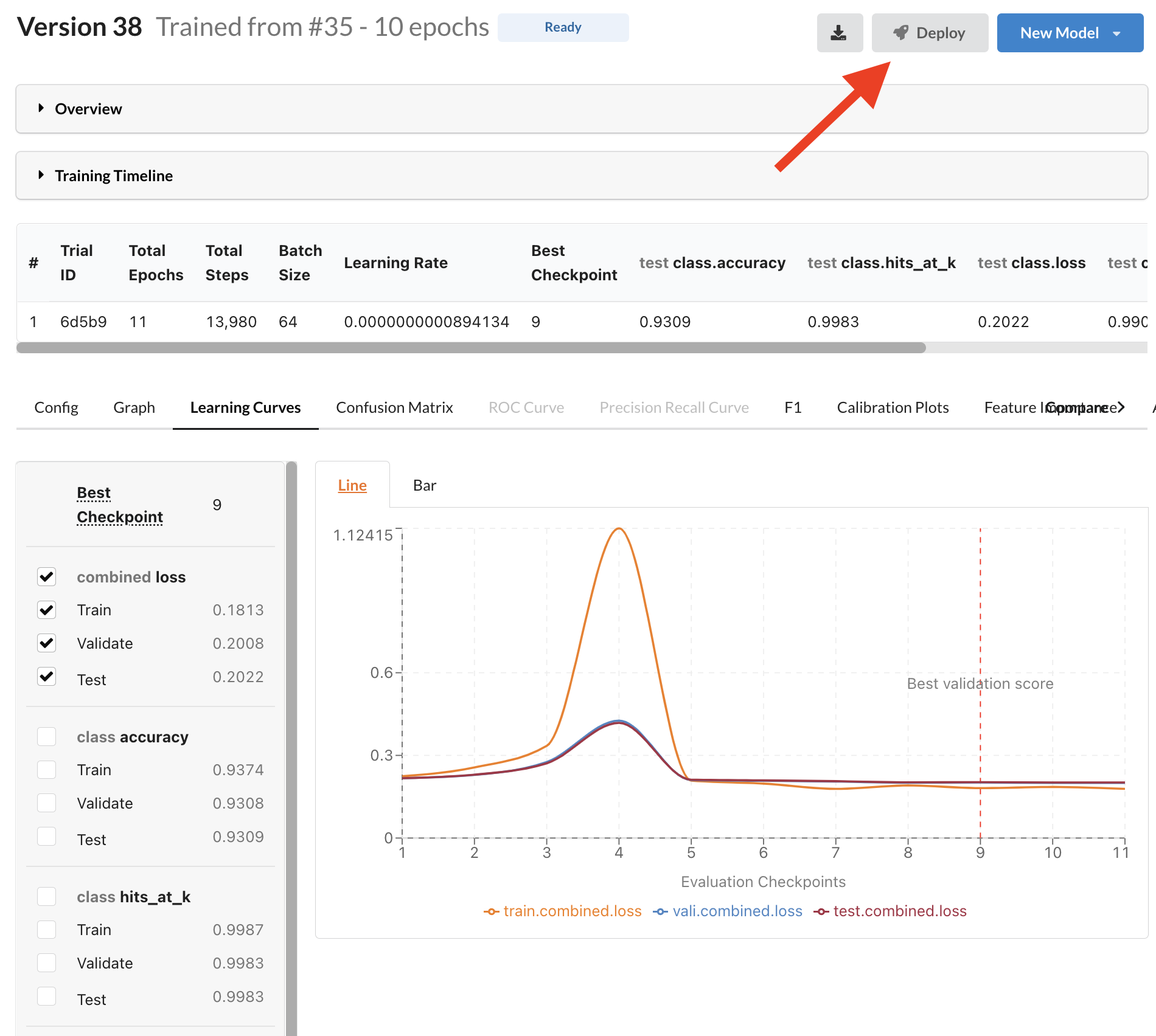
Deploy in minutes for real-time or batch inference by clicking the deploy button.

Summary

Today we tried a total of 8 models. We started with the default neural network, and then tried the 6 models from Predibase’s suggested models. Out of the 6 models, we found that the pre-trained BERT with finetuning performs the best, but it was overfitted. To fix it, we reduced the learning rate and arrived at the final model. The accuracy of test and train in the final model is slightly lower than the previous one, but model will be more robust with new data because it’s not overfitted. 

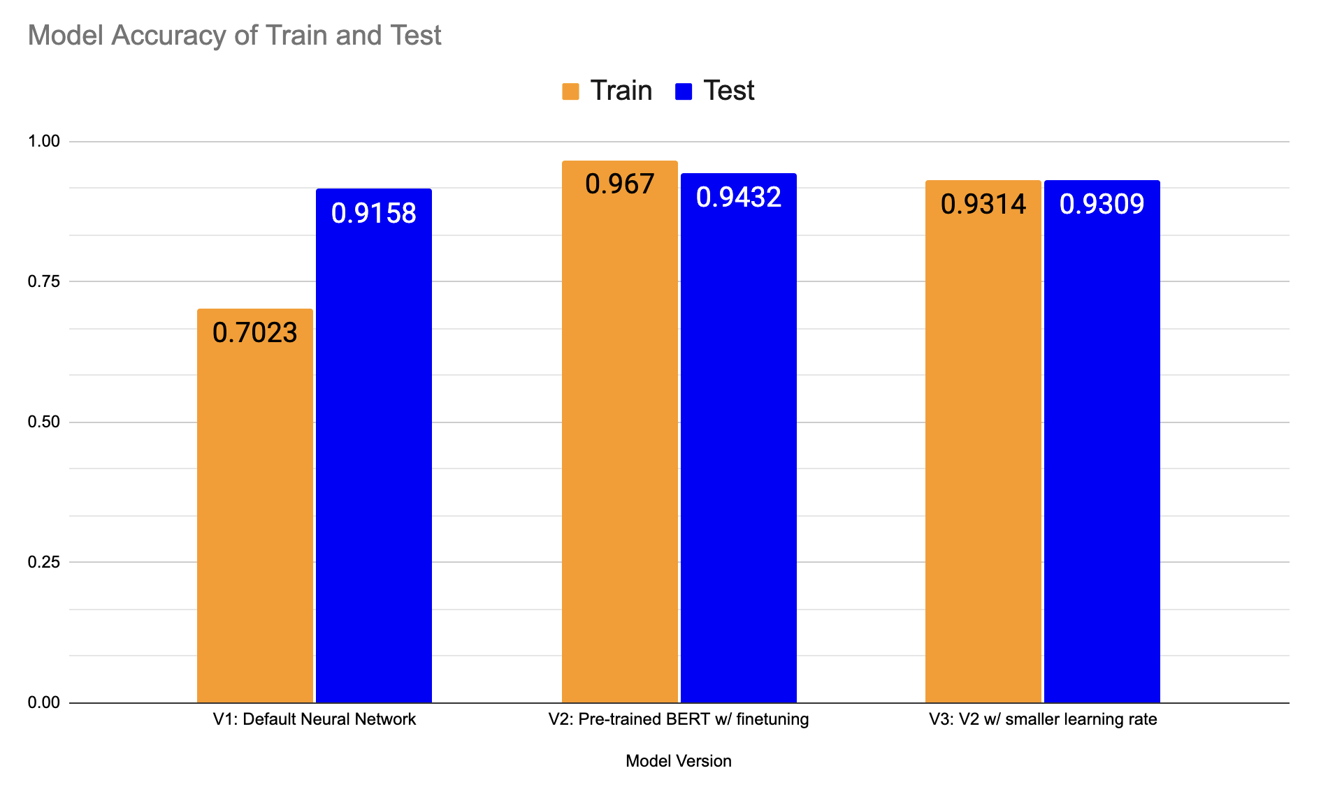
Comparing performance of our final text classification models.

Getting Started with NLP on Predibase

In this example, we showed you how to build an end-to-end ML pipeline for topic classification in less than 10 minutes using state-of-the-art deep learning techniques on unstructured data with Predibase. This was possible due to the underlying compositional Encoder-Combiner-Decoder (ECD) model architecture that makes unstructured data as easy to use as structured data. This is powerful for any enterprise  looking to automate the labeling of unstructured text documents.

This was also just a quick preview of what’s possible with Predibase, the first platform to take a low-code declarative approach to machine learning. Predibase democratizes the approach of Declarative ML used at Big Tech companies, allowing you to train and deploy deep learning models on multi-modal datasets with ease. 

If you’re interested in finding out how Declarative ML can be used at your company:

• Request a custom demo of Predibase to get started building your own models
• Try this model using our open source project Ludwig with this Jupyter Notebook