Introduction to Fraud Detection with Declarative Machine Learning

As financial fraud has become increasingly sophisticated, with rapidly changing patterns that make detection difficult for financial institutions, machine learning has emerged as a powerful tool to detect fraudulent patterns.

In this tutorial, we'll show you how to build an end-to-end fraud detection model using Predibase, the low-code AI platform, and the open-source project Ludwig. Specifically, we will discuss how to connect data, rapidly build and iterate on ML models in a declarative way, compare results and explore techniques for dealing with class imbalance. You can get started building this on your own with a free trial of Predibase or trying it out with this Ludwig notebook

Detecting Credit Card Fraud with Machine Learning 

Fraud detection poses a challenge as fraudulent examples are scarce compared to normal transactions, causing the dataset to be highly imbalanced. However, by analyzing extensive data, machine learning algorithms can identify patterns and anomalies that could signify fraudulent behavior.

Credit Card Fraud Dataset

For this tutorial, we are going to use the Credit Card Fraud dataset hosted on Kaggle. The dataset contains transactions made by credit cards in September 2013 by European cardholders.

We will be working with a dataset that contains information on transactions that occurred over two days. Out of 284,807 transactions, only 492 were identified as fraudulent. This makes the dataset highly unbalanced, as the positive class (frauds) only make up 0.172% of all transactions.

It contains only numerical input variables which are the result of a PCA transformation. Due to confidentiality issues, we cannot provide the original features and more background information about the data. Features V1, V2, … V28 are the principal components obtained with PCA, the only features which have not been transformed with PCA are 'Time' and 'Amount'. Feature 'Time' contains the seconds elapsed between each transaction and the first transaction in the dataset. The feature 'Amount' is the transaction Amount, this feature can be used for example-dependent cost-sensitive learning. Feature 'Class' is the response variable and it takes value 1 in case of fraud and 0 otherwise.

You can use Predibase’s PQL Query Editor to quickly check the distribution of the data using SQL-like commands as shown below:

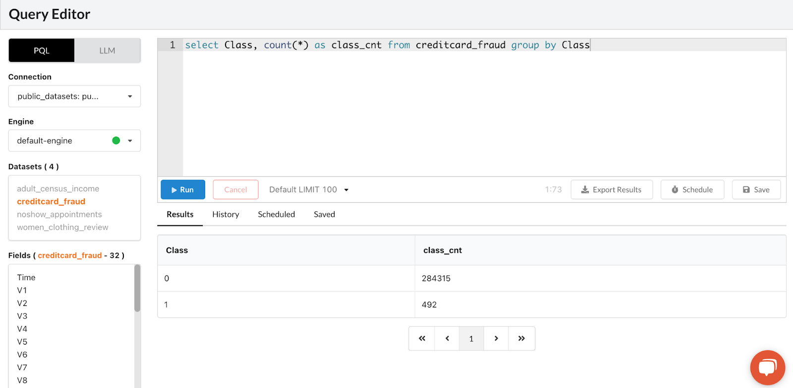
Check the distribution of your data with SQL like commands using Predibase's Predictive Query Editor

Step 1: Connecting Public Fraud Dataset

Predibase allows you to instantly connect to both your local directory and cloud data sources, pulling in all your data—including tabular, text, images, audio, and more—wherever it may live. For today’s example, we are going to use a public fraud dataset located in Ludwig’s datasets by clicking “Public Datasets”.

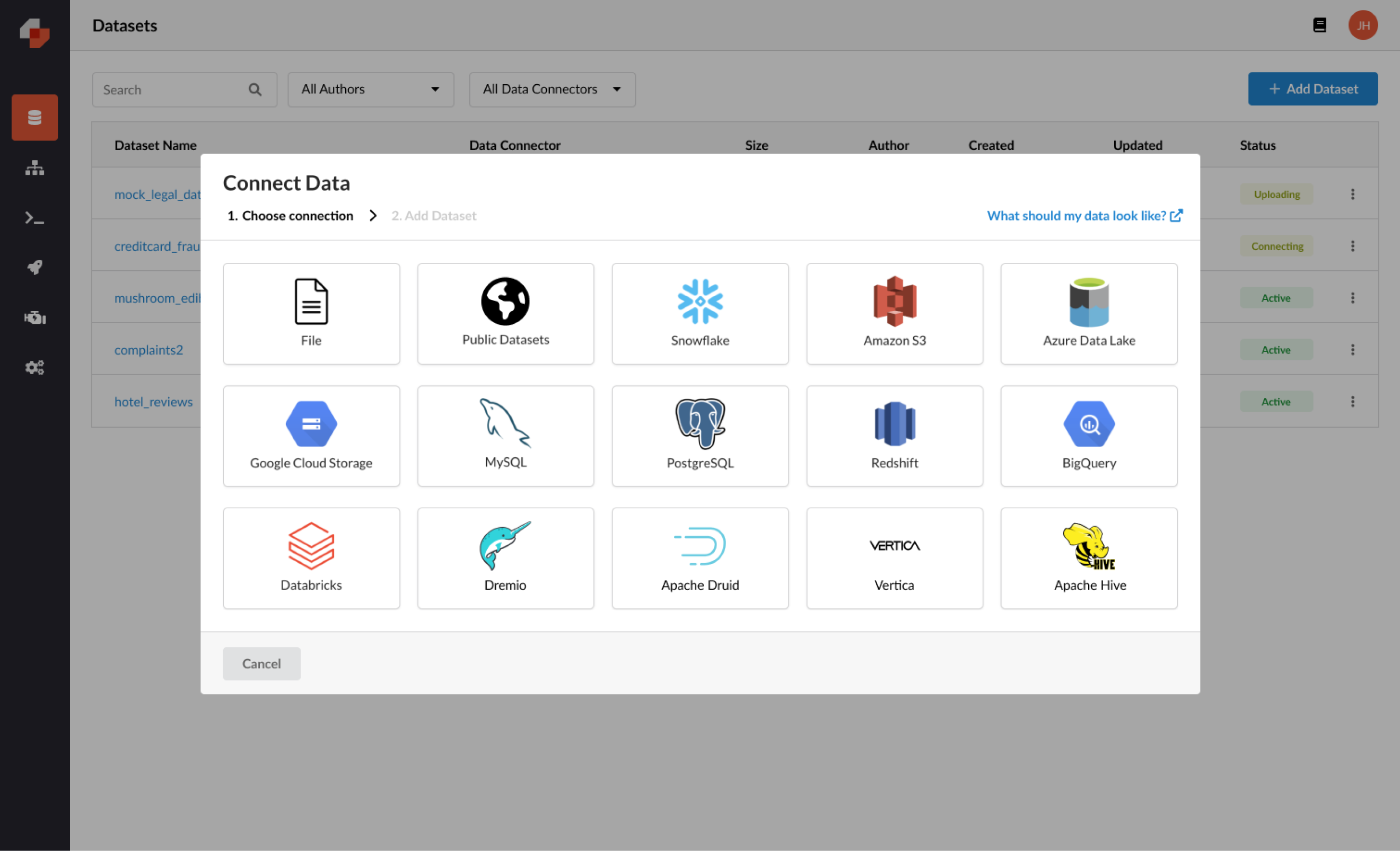
Connecting data is as easy as one click in Predibase

Step 2: Building our first fraud detection model with a neural network

Before we build our first model, let me explain how Predibase works. Predibase is the first platform to take a low-code declarative approach to machine learning. Instead of writing thousands of lines of code, you can build state-of-the-art models with concise but flexible configurations. Declarative ML systems have been adopted by leading tech companies Apple, Meta, and Uber and Predibase is the first ML platform to make this approach available to all enterprises.

The algorithms used in Predibase are based on the open-source Ludwig framework originally developed at Uber (8,800+ stars on GitHub). With Ludwig, all you have to do is specify your input and output features in a configuration-driven manner—in this case, YAML—to start to train your baselines. Predibase simplifies this modeling process even further, reducing the process to arrive at a trained model to just a few clicks. 

Want to see declarative ML in action? Let’s train our first model to see how it works.

If you don’t know what kind of configuration is best for your first model, Predibase will suggest one based on your specific dataset by selecting “Basic defaults”.

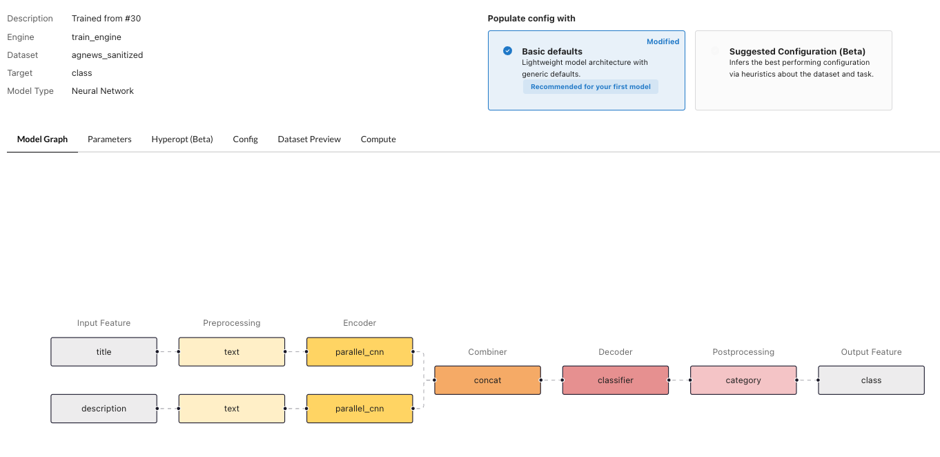
Predibase automatically generates a suggested neural network model architecture for your first fraud model

At Predibase, we compose and visualize a suggested model architecture for you. For example, you can see that we use parellel_cnn as an encoder for input features, and the outputs go through a concat combiner. The concat combiner consumes all outputs from encoders. It concatenates and then optionally passes the concatenated tensor through a stack of fully connected layers. If you’re curious to learn more about the Encoder-Combiner-Decoder (ECD) architecture, you can read about Ludwig’s architecture here.

Based on the data, Predibase suggests this config to get your first trained model:

- name: V11
    type: number
  - name: V19
    type: number
…
  - name: V28
    type: number
  - name: Amount
    type: number
output_features:
  - name: Class
    type: binary
output_features:
  - name: Class
    type: binary
combiner:
  type: concat

Initial fraud model results

You can simply click train to kick off model training. Predibase manages the infrastructure for model training and will right-size the compute resources based on the size and properties of your dataset. When it’s ready, you will have access to various model performance metrics as well as the hyperparameters used for training. 

Let’s take a look at the learning curve. It looks like the loss of the validation set and test set converged. Since this is a dataset with highly imbalanced classes, the accuracy metric doesn’t matter in this case, and we will mainly use the Precision-Recall Curve (AUPRC or PR Curve) as the main metric to evaluate the model. The precision is 0.85 and the recall is 0.573.

Here is a quick review of the concepts of precision and recall (you can skip this part if you are familiar with these concepts):

Precision in this context measures how many of the transactions flagged by the model as fraudulent were actually fraudulent. For example, if the model flagged 100 transactions as fraudulent, and 90 of them were actually fraudulent, then the precision would be 90%.

Recall, on the other hand, measures how many of the actual fraudulent transactions are correctly identified by the model. For example, if there were actually 200 fraudulent transactions, and your system correctly identified 90 of them, then the recall would be 45%.

In an imbalanced dataset, where the number of fraudulent transactions is much lower than the number of legitimate transactions, precision and recall become particularly important. A model that simply flags all transactions as legitimate would have high accuracy but would fail to detect any fraudulent transactions. By considering precision and recall, you can better evaluate the effectiveness of your fraud detection system and make improvements where necessary.

Although the AUROC curve below looks good, the Precision-Recall curve doesn’t perform very well for this model given the recall being 0.573.

Learning Curve

Initial learning curve for our fraud detection model

Confusion Matrix

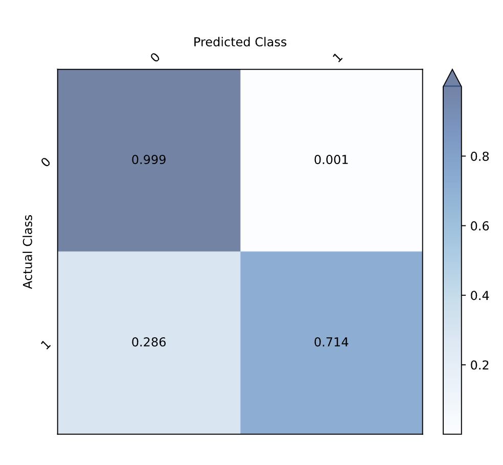
Confusion matrix for our first fraud model

AUROC Curve

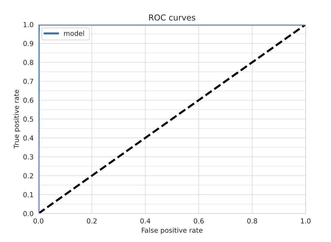
AUROC curver for our first fraud model

Precision-Recall Curve

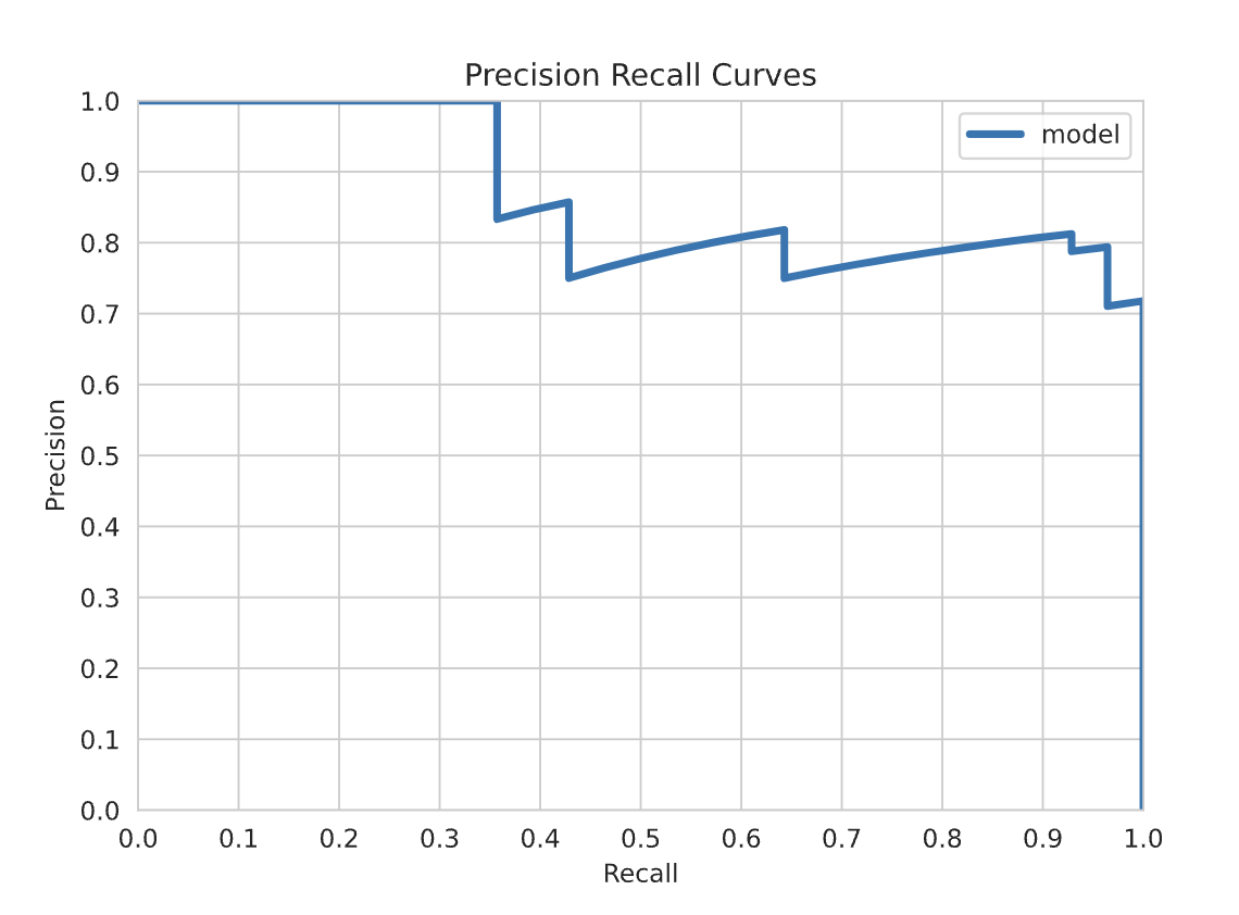
Precision-Recall Curve for our first fraud model

Let’s try some different models to see if we can improve our precision and recall.

Step 3: Exploring suggested models including LightGBM

In the early stage of model development, it’s helpful to try a few different models and see what works well. With Predibase, you don’t need to set up those experiments manually, you can simply select “Explore suggested models”. For tabular datasets, this will give you 6 models including a default neural network (ECD) and LightGBM which performs well on tabular datasets.

Easily train a series of recommended models with an AutoML approach using Predibase

If you are not familiar with the ECD and LightGBM, let me quickly explain.  

Ludwig’s core modeling architecture is referred to as ECD (encoder-combiner-decoder). Multiple input features are encoded and fed through the Combiner model that operates on encoded inputs to combine them. On the output side, the combiner model's outputs are fed to decoders for each output feature for predictions and post-processing. Learn more about Ludwig's architecture here.

When visualized, the ECD architecture looks like a butterfly and sometimes we refer to it as the “butterfly architecture”. The architecture allows you to automatically generate models for any number of use cases.

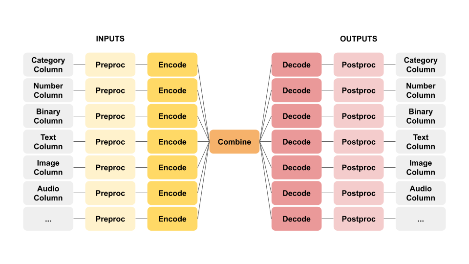
The ECD architecture supports many different machine learning use cases in a single unified architecture.

Building GBM Models in Predibase

Predibase uses a compositional architecture (ECD) with neural networks as the default for modeling. This is because neural networks are able to handle a wide range of data types and support multi-task learning, making them a versatile choice for many applications.

While neural networks work well with many types of data, they are relatively slow to train and they may not always be the best choice for tabular data, particularly when the dataset is small or when there is class imbalance. Additionally, using multiple frameworks to try different model types can be time-consuming and cumbersome.

One of the key advantages of gradient-boosted trees is their speed of training compared to neural network models. They also tend to perform competitively on tabular data and be more robust against class imbalance compared to neural networks, making them a reliable and widely-used tool among practitioners. By adding gradient-boosted trees, we hope to provide you with a unified interface for exploring different model types and obtain improved performance in particular on small tabular data tasks. Under the hood, Ludwig uses LightGBM to train a gradient boosted tree model. LightGBM is a gradient boosting framework that uses tree based learning algorithms and is designed to be scalable and performant. We created an interactive tutorial that you can explore here.

Don’t worry if you don’t know the details of architectures of the models we use, we make it easy for you to run experiments on Predibase without needing deep machine learning knowledge. Let’s kickstart the set of suggested models and see which one performs the best!

Fraud model results

After all 6 models have finished training, we found that the GBM model performs the best. This is the config suggested by Predibase:

- name: V1
    type: number
  - name: V2
    type: number
…
  - name: V28
    type: number
  - name: Amount
    type: number
output_features:
  - name: Class
    type: binary
output_features:
  - name: Class
    type: binary
defaults: {}
model_type: gbm

Let’s look at the learning curve again. It looks like the loss of validation and test set also converged. The Precision-Recall Curve looks much better this time.

The precision is 0.9067 and the recall is 0.764. For a dataset with very imbalanced data, this is a good baseline model we can use.

Learning Curve

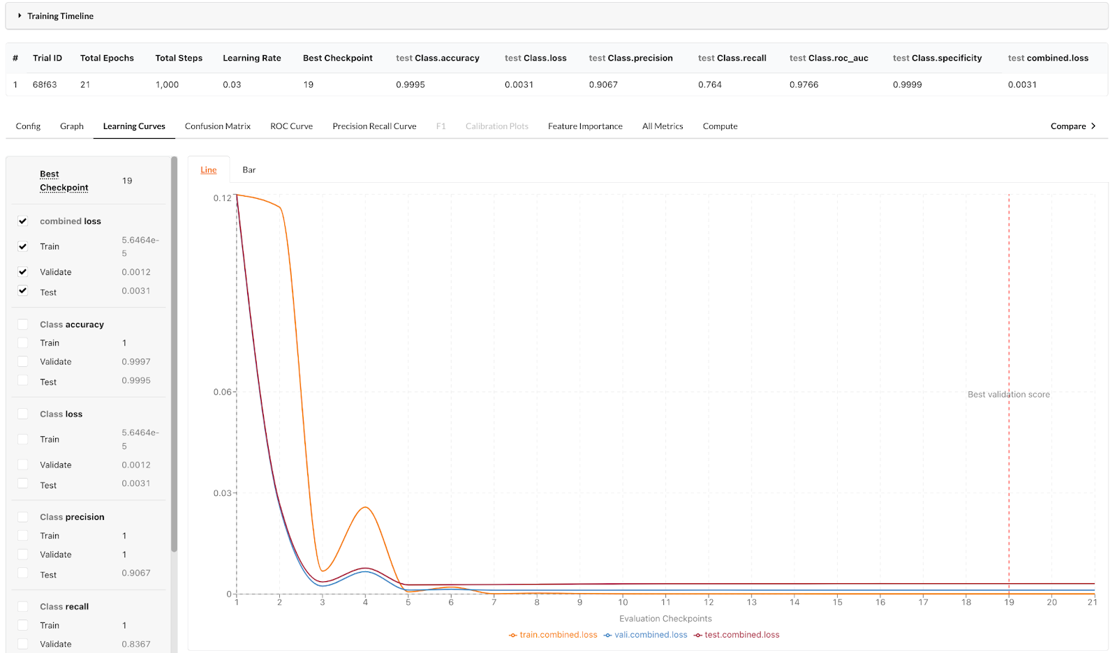
Learning curve for our GBM model

Confusion Matrix

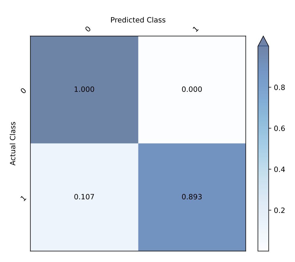
Confusion Matrix for our GBM model

AUROC Curve

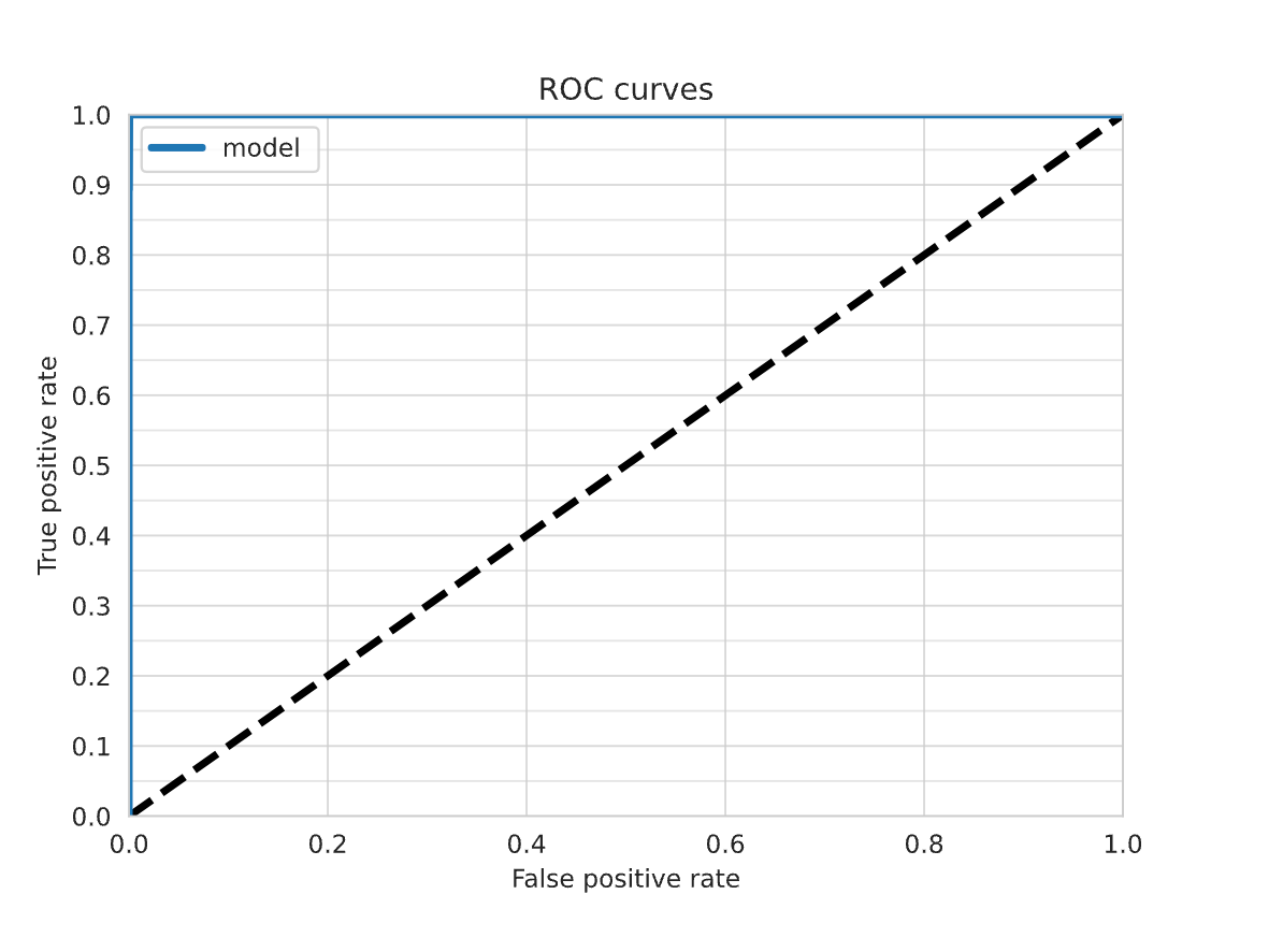
AUROC Curve for our GBM model

Precision-Recall Curve

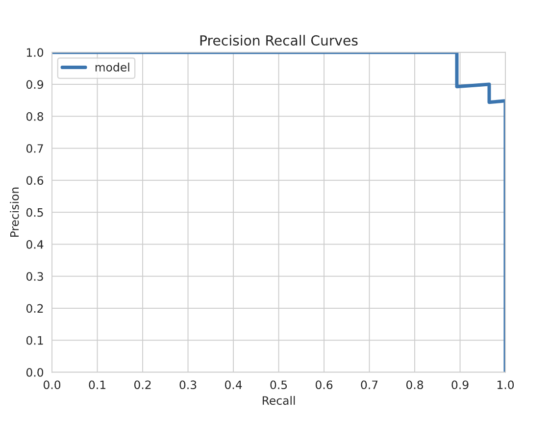
Precision-Recall Curve for our GBM model

Three additional techniques to deal with class imbalance

If you want to further improve your model with an imbalanced dataset, here are three techniques we recommend and you can easily implement them in Predibase.

1. Upsampling and downsampling

You can change the parameters in “Oversample Minority” or “Undersample Majority”.

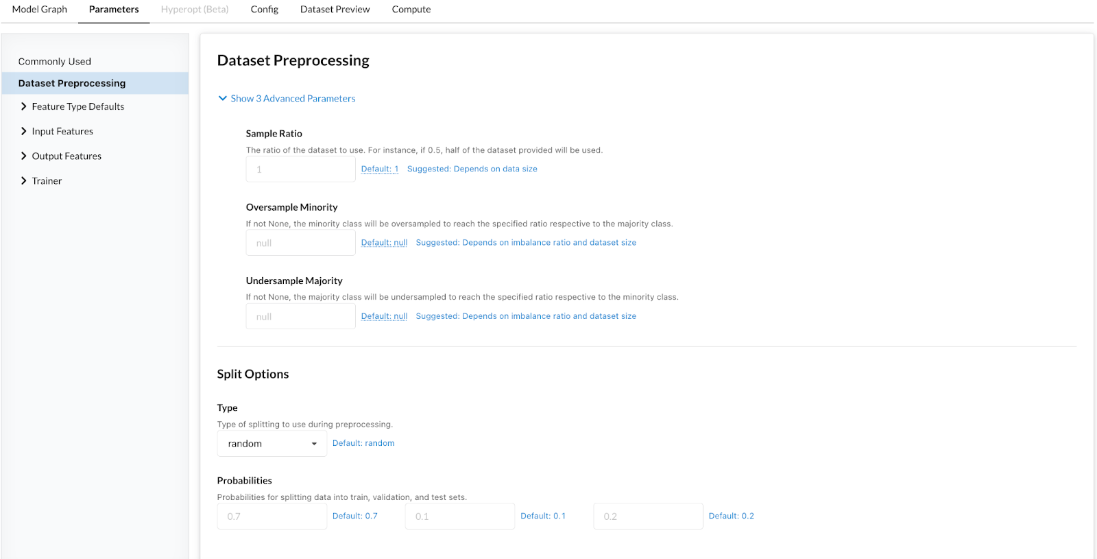
In a few clicks, you can change the model parameters to oversample or undersample your dataset.

2. Stratified sampling

You can select “stratify” in the “Type” drop-down of the “Split Options”.

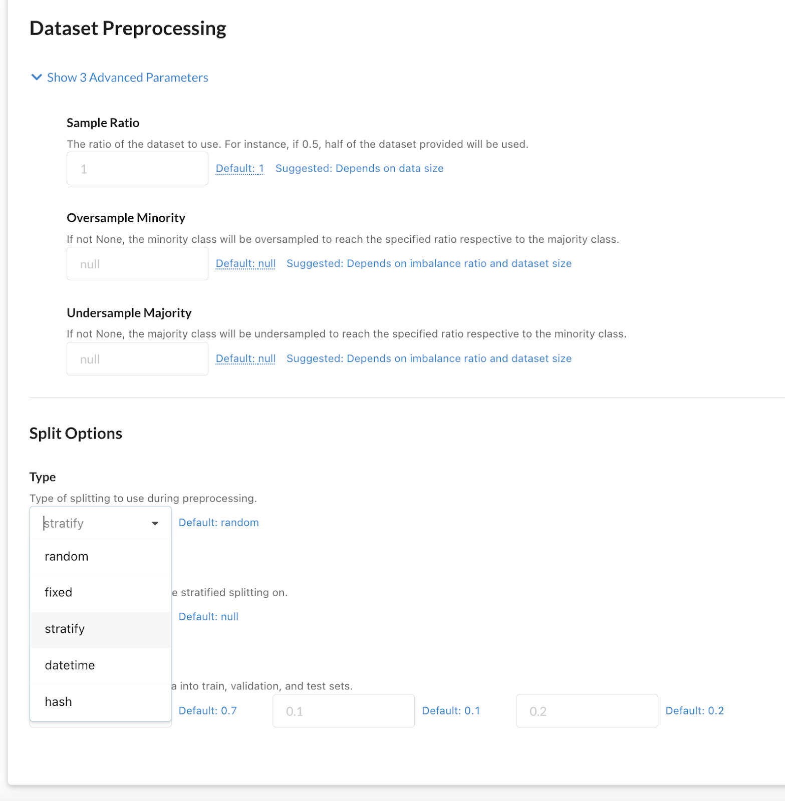
Change model parameters for stratified sampling in one click.

3. Change class weights

In the “Output Features” section, you can select a “Positive Class Weight” to change how the loss function is calculated.

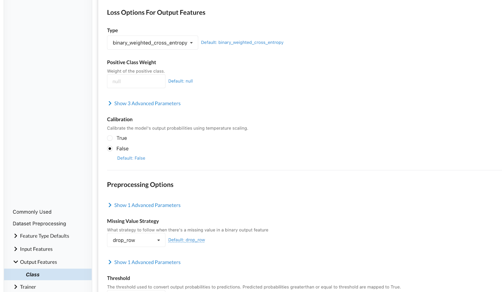
Change class weights to improve model performance.

Summary of our fraud model results

First, we used the default neural network model to train a fraud detection model and the recall wasn’t good enough. Then we tried another six model architectures recommended by Predibase and the LightGBM model performed well on both precision and recall. We also shared three additional techniques for you to try on your imbalanced datasets.

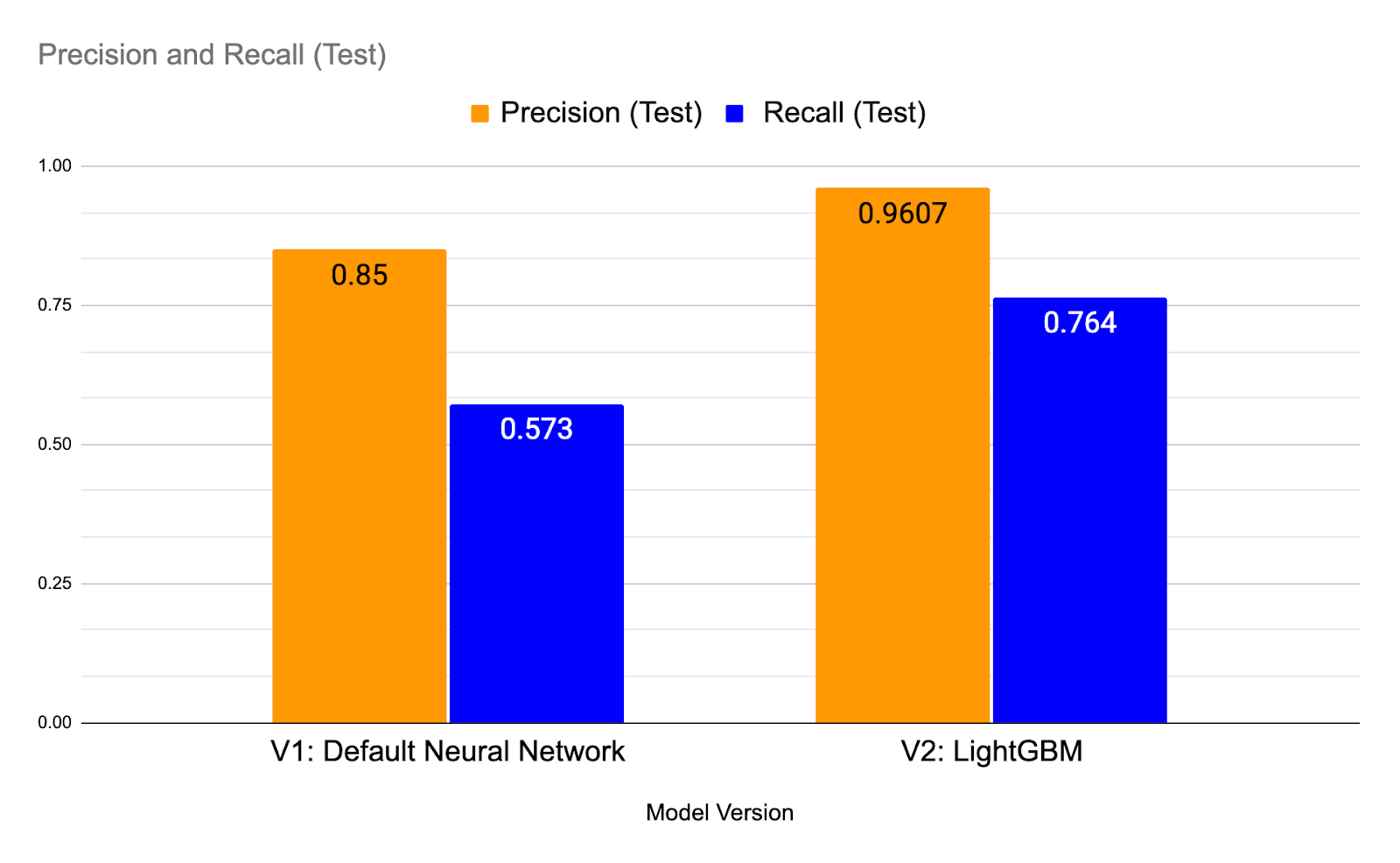
Comparing our fraud models to determine if the neural network or GBM performed better for Precision and Recall.

Get started building fraud models on tabular data with declarative ML

In this example, we showed you how to build an end-to-end ML pipeline for credit card fraud detection in less than 10 minutes using state-of-the-art deep learning techniques on tabular data with Predibase. This was possible due to the underlying compositional Encoder-Combiner-Decoder (ECD) model architecture and the option of using LightGBM, which makes it easy to explore different models for tabular data. This example also showcased Predibase’s ability to tackle imbalanced datasets.

This was just a quick preview of what’s possible with Predibase and Ludwig, the first platform to take a low-code declarative approach to machine learning. Predibase democratizes the approach of Declarative ML used by big tech companies, allowing you to train and deploy deep learning models on multi-modal datasets with ease. 

If you’re interested in finding out how Declarative ML can be used at your company:

• Build this model in Predibase by signing up for a free trial.
• Use our open source project Ludwig along with this Jupyter Notebook for fraud detection.
• Watch our fraud detection demo video to follow along.