In today's rapidly evolving AI landscape, software engineers and developers are facing growing expectations to integrate machine learning (ML) into their products. However, grasping the fundamentals of ML can pose a significant challenge. That's why we started a new series of tutorials for the ML-curious engineer that contain practical advice and best practices for working with ML models.
In this first post, we dive into one of the most widespread challenges: overfitting. We’ll use open source declarative ML framework Ludwig and Predibase to demonstrate how to address and avoid overfitting. You can follow along with this tutorial by signing up for a free trial of Predibase.
What is overfitting in machine learning?
When a model has “overfit”, it means that it has learned too much about the training data and is unable to generalize what it has learned to a new set of unseen data.
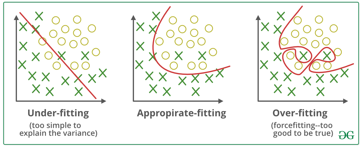
Visualization of underfitting and overfitting in ML from https://www.geeksforgeeks.org/underfitting-and-overfitting-in-machine-learning/
Signs of an Overfit Model
You can identify an overfit model by comparing performance metrics on training and validation datasets. A key method is to analyze loss vs iterations plots:
- If training loss keeps decreasing while validation loss begins to rise, your model is likely overfitting.
- A large gap between training and validation accuracy is another red flag.
Diagnosing overfitting in practice
It is easy to identify overfitting by inspecting the model’s performance metrics across its training and validation sets. The symptom for overfitting is increasingly strong performance on the training set in contrast to stagnant or declining performance on the validation and test sets.
An example of this can be found below. The model whose learning curves are shown below is trained on the Adult Census dataset, a dataset composed of tabular data. The model’s task is to classify each person's income as either below or above $50,000 based on their attributes as collected by the US Census.
Here, we see that the training loss (orange) is steadily decreasing over time and that the validation and test loss (blue and red) is increasing over time. What this typically means is that the model has stopped learning generalizable features from the data and begun exploiting details and noise specific to the samples of the training set to determine income. This exploitation leads to a boost in its accuracy on the training set and is a primary indicator of overfitting.

Example of a learning curve that shows overfitting
How to prevent overfitting
Fixing overfitting means preventing the model from learning associations that are specific to the training set. There are two common ways to fix overfitting: modifying the training set or regularizing the model.
1. Modifying the training set
You can modify the training set of the data in order to ensure that the model is best set-up for success during the training process. It helps improve model performance and generalization by introducing variations and diversifying the data, making the model more robust and better able to handle real-world scenarios.
Data augmentation, a technique in machine learning that expands the training dataset by creating modified versions of existing data, is an example of a method used to reduce the likelihood of overfitting. Data augmentation helps improve model performance and generalization by introducing variations and diversifying the data, making the model more robust and better able to handle real-world scenarios.
That said, oftentimes it is impossible to modify the data in a meaningful way, typically because data acquisition costs are too high. In these cases, we can turn to an approach called “regularization”, which makes tweaks to the model itself to prevent overfitting.
2. Regularizing the model
Broadly, regularization is a mechanism we can add to the model training process to handicap the model’s ability to memorize the little details that may be found in the training set. This becomes particularly relevant for Deep Neural Networks, which may have billions of parameters and therefore the capacity to memorize massive amounts of data.
2.1 Controlling Growth (Trees only)
Decision trees are often regularized by limiting the branch creation process. Typically, a decision tree becomes overfit if its branches become too specific to particular examples in the training set. Below are some ways to prevent this in decision trees:
- Enforcing a maximum tree depth in the overall decision tree.
- Enforcing a maximum number of leaves in the overall decision tree
- Enforcing a minimum number of data points per leaf
You can edit those parameters in Ludwig when using the tree-based models (model_type: gbm) by setting max_depth, num_leaves, min_data_in_leaf. More about gbm models parameters in Ludwig can be found here.
To adjust these values in Predibase, go to the Trainer -> General section.
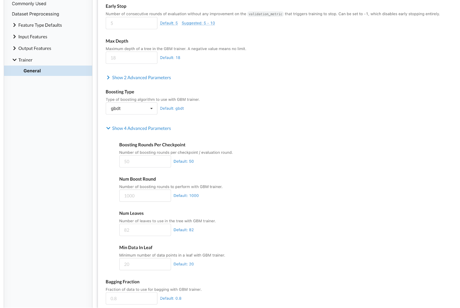
Adjusting tree model parameters in Predibase is a easy as a few clicks
2.2 Weight Decay
Both neural networks and decision trees support a regularization method known as “weight decay”– simply put, weight decay limits how large the weight values can be within a particular ML model. Generally, the values of a model’s weights are how the model formulates its decisions about its inputs.
By enforcing weight “sparsity” within the model during training, the model is limited in how sensitive it can be to particular features for a given sample. This limitation encourages it to focus on only the most important features across all samples, therefore preventing overfitting.
Typically, weight decay is controlled by some lambda coefficient, which describes how strongly you want to enforce the sparsity constraint in your architecture. Higher values indicate stronger regularization.
To adjust this value in Ludwig, set the Regularization Lambda under Trainer. Some good values to try for this parameter are 0.0001, 0.001, 0.01, and 0.1.
To adjust this value in Predibase, search for Regularization Lambda in the Parameters tab of the Model Builder.
2.3 L1 and L2 Regularization
Both L1 and L2 regularization techniques introduce a regularization term that penalizes the model for having large coefficients. By adding this penalty, the model is discouraged from relying heavily on any single feature and instead encouraged to find a balance among all features. This helps prevent overfitting by reducing the complexity and variance of the model, leading to improved generalization on unseen data.
L1 regularization promotes sparsity and feature selection, while L2 regularization encourages smaller but non-zero coefficients. L1 regularization can help in selecting the most relevant features and reducing model complexity. L2 regularization helps in reducing the impact of less important features on the model's predictions, resulting in a more stable and generalized model.
These regularization techniques play a vital role in preventing overfitting and improving the overall performance and generalization capability of machine learning models. The choice between L1 and L2 regularization depends on the specific problem, the nature of the data, and the trade-off between interpretability and complexity.
In Ludwig and Predibase, you can set regularization_type as L1 or L2.
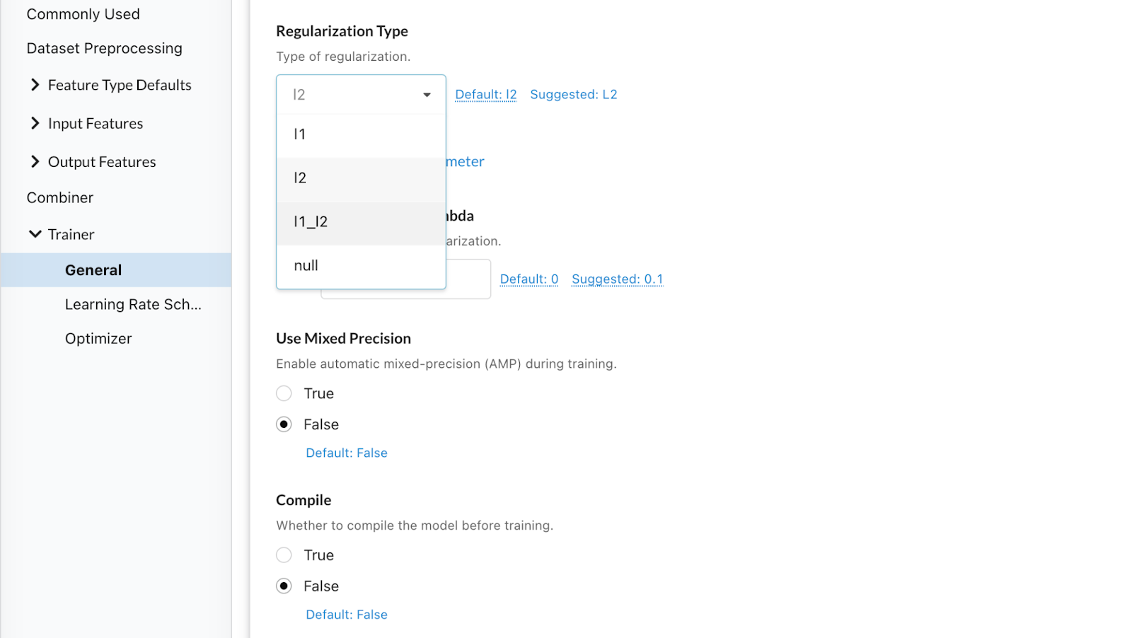
Adjusting regularization in Predibase
2.4 Dropout
Both neural networks and some types of decision trees (e.g. DART) support another regularization method known as “dropout”. Dropout is a mechanism enabled during the training process that will temporarily “drop” components of the model architecture at random during training. For neural networks, the components are typically individual neurons. For DART models, the components are typically individual trees.
By dropping these components, the overall model is operating at only a fraction of its total capacity at any given moment. This limitation forces the model to reduce its reliance on any one component and build redundancy into its architecture. This in turn limits its capacity for memorizing too many fine details about samples in the training set, thus preventing overfitting.
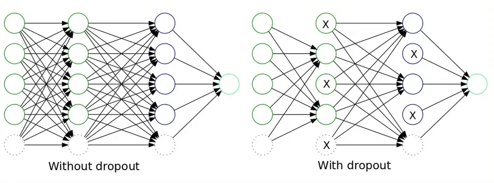
Applying dropout in a neural network from https://dotnettutorials.net/lesson/dropout-layer-in-cnn/
Typically, dropout is controlled by the probability of dropping components. Higher values mean that components are dropped more frequently during training, and thus cause stronger regularization.
To adjust dropout rate in Ludwig, use dropout_rate.
To adjust this value in Predibase’s model builder using “Basic defaults”, go to Parameters ->Combiner-> Dropout (as below). Some good values to try for this parameter are 0.1, 0.2, and 0.5.
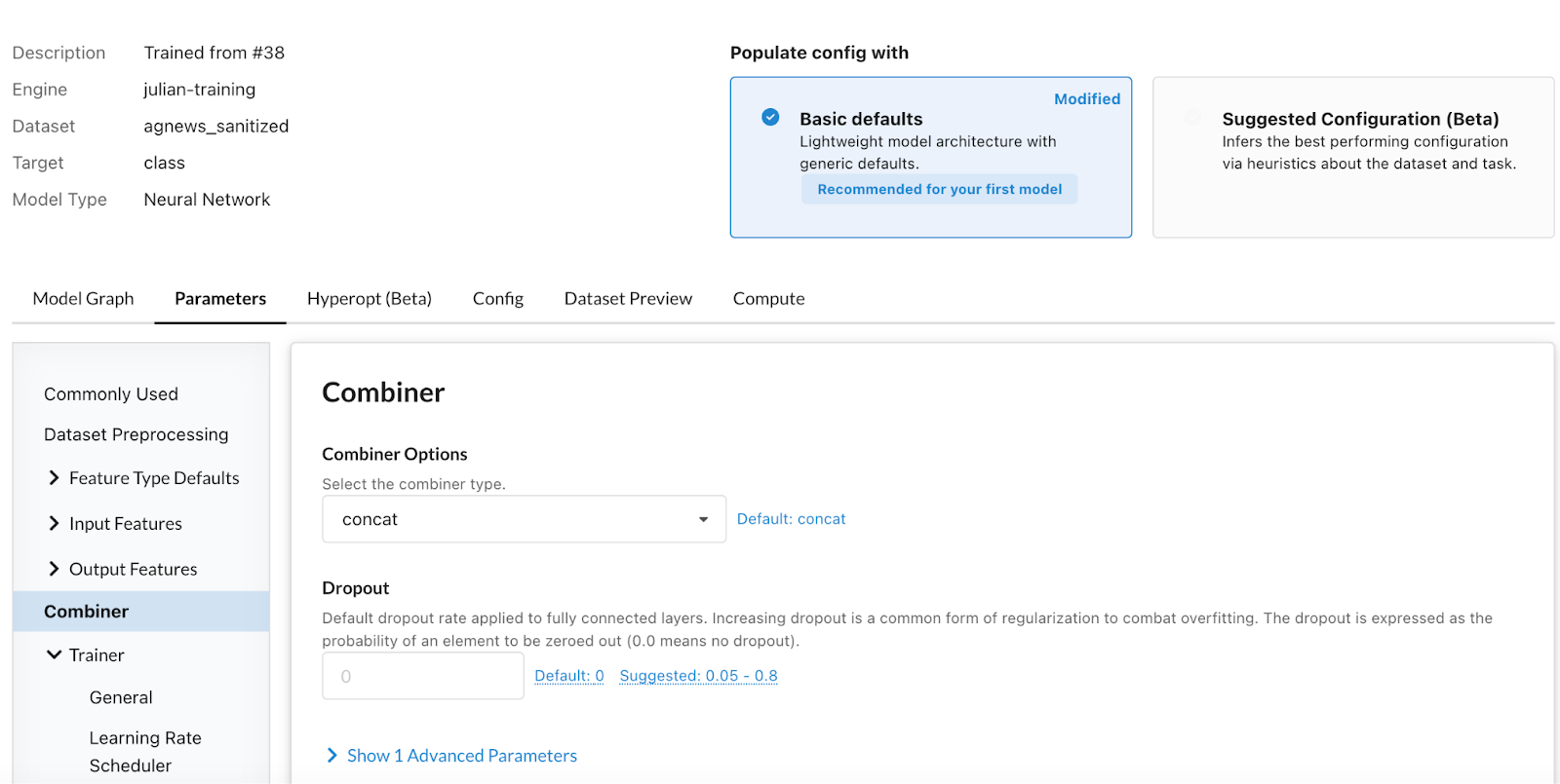
Adjusting drop-out in Predibase
2.5 Smaller batch size
In Chapter 6 of Goodfellow's deep learning book:
Small batches can offer a regularizing effect (Wilson and Martinez, 2003), perhaps due to the noise they add to the learning process. Generalization error is often best for a batch size of 1. Training with such a small batch size might require a small learning rate to maintain stability because of the high variance in the estimate of the gradient. The total runtime can be very high as a result of the need to make more steps, both because of the reduced learning rate and because it takes more steps to observe the entire training set.
In Ludwig, you can set the Batch Size under the Trainer section.
In Predibase’s model builder, under “Basic defaults”, go to Parameters -> Commonly Used-> Batch Size (as below) to adjust it.
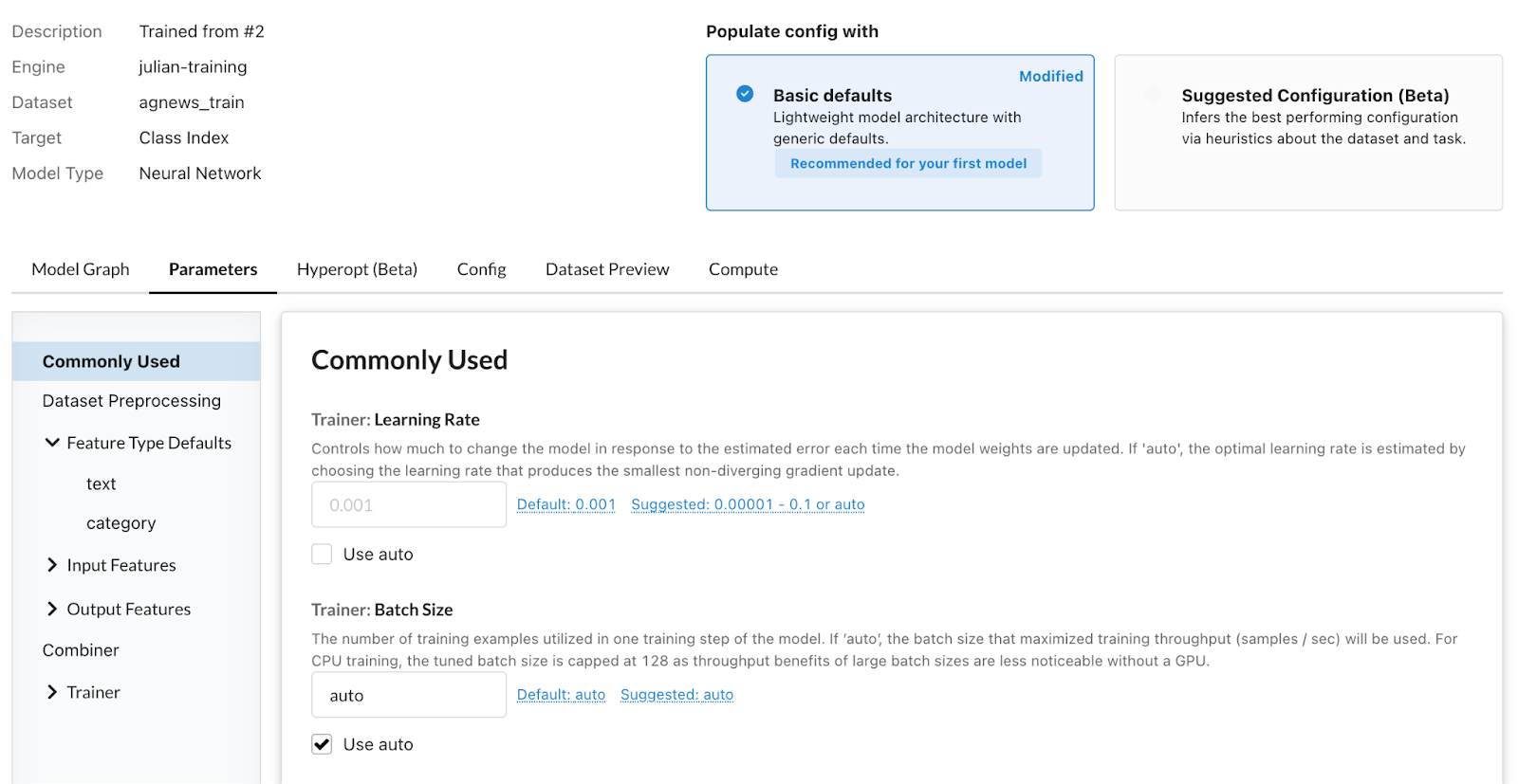
Changing batch size in Predibase
2.6 Early Stopping
Early stopping entails monitoring the performance of the model on a validation set while. it undergoes training. If the model's performance shows signs of deterioration, the training process is stopped before overfitting occurs. This approach prevents unnecessary iterations and aids in finding the optimal balance between underfitting and overfitting.
In Ludwig, you can use the early_stop parameter under trainer to determine when you want the training to stop.
In Predibase’s model builder, under “Basic defaults”, go to Parameters ->Trainer-> Epochs (as below) to limit how many epochs you want the model to train.
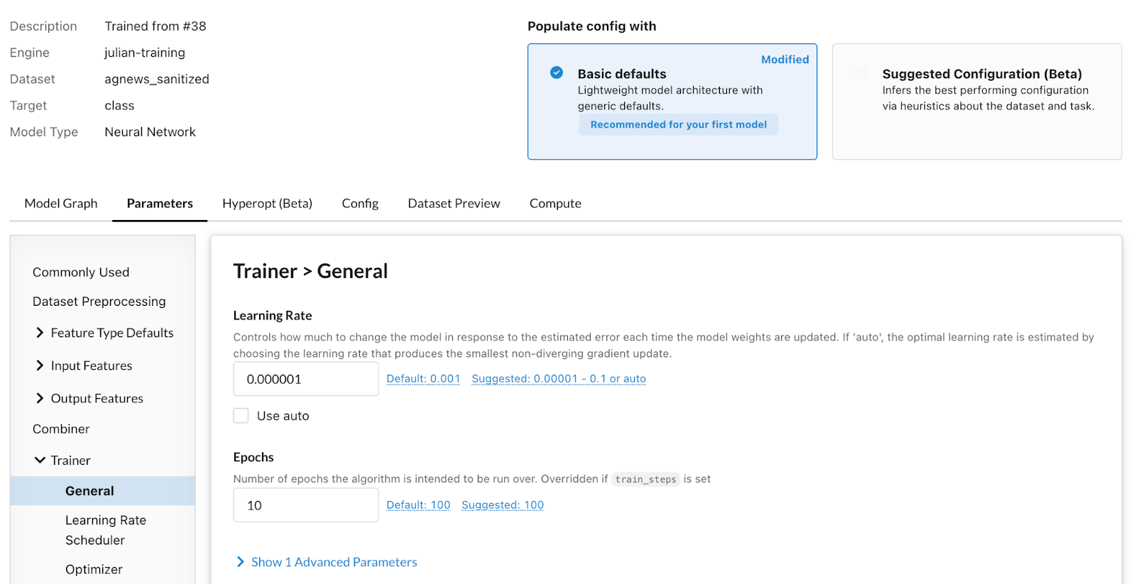
Limit how many epochs you want the model to train
2.7 Normalization
Neural networks have mechanisms that prevent overfitting without having been designed for it. An example is normalization (batch, layer, cosine, and other kinds) normalize the values of activations. This in turn makes it so that the absolute value for the parameters at the following layers does not have to be very large or very small to account for very large values in the activations. Implicitly, this regularizes the weights and makes gradients less prone to explode or vanish through the layers.
In Ludwig, you adjust this value by setting the norm parameter under combiner to either batch or layer.
To adjust this value in Predibase, search for Norm in the Parameters tab of the Model Builder and go to the Combiner section.
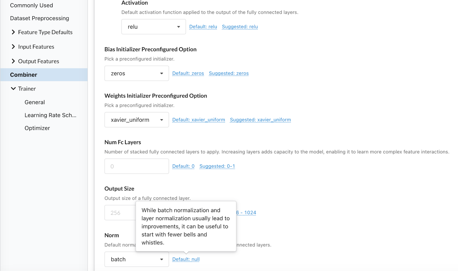
Adjusting model normalization
Can you completely avoid overfitting?
it is normal that your train accuracy is little higher than your test accuracy. Your model possesses an inherent advantage when it comes to the training set as it has already been provided with the correct answers.
Is overfitting always bad?
While overfitting is an indicator that your model is not as performant as it could ultimately be, it is often a good signal during the modeling process that you are on the right track.
One practice commonly seen in the machine learning development lifecycle is actually striving for overfitting as a modeling milestone. Once you have a model that is capable of getting strong performance on the training set, you likely have a model with sufficient expressive capacity to learn the broader strokes required to attain good generalization performance on its validation set and beyond.
Careful application of the regularization techniques listed above will typically yield stronger performance in such cases, and bring you closer to your model quality acceptance criteria.
Ready to train a model with just a few lines of code?
Get started with a free trial of Predibase to train your model and use the tips above to see if you can avoid overfitting.
FAQs
What is overfitting in machine learning?
Overfitting in machine learning occurs when a model learns the training data too well—including its noise—resulting in poor performance on new, unseen data. The model fits the training set tightly but lacks generalization.
How does increasing model complexity lead to overfitting?
Increasing model complexity, such as adding more parameters or layers, can cause the model to fit the training data too closely, capturing noise and reducing its ability to generalize.
What are common techniques to prevent overfitting in neural networks?
To prevent overfitting, you can use regularization techniques (like L1/L2), cross-validation, dropout in neural networks, data augmentation, or simply reduce model complexity. Early stopping based on validation loss is also effective.
How can I identify if my model is overfitting?
You can detect an overfit model by comparing training and validation loss. If training loss continues to decrease while validation loss increases, it's a sign of overfitting. This is often visible in a loss vs iterations plot.
What does loss vs iterations tell us about overfitting?
The loss vs iterations graph shows how the model performs during training. If training loss keeps decreasing but validation loss starts increasing, it’s a clear indicator of overfitting.
